DINOv2: How self-supervised visual features transfer across tasks

Image classification needs a compact description of an entire image. Segmentation and depth estimation need a useful description at every patch. Retrieval needs features that place visually related images close together even when style, pose, or background changes.

DINOv2 tackles these requirements with one Vision Transformer encoder. It combines image-level self-distillation, masked patch prediction, a feature-spreading regularizer, curated data, and engineering at scale. The released family spans ViT-S/14, ViT-B/14, ViT-L/14, and ViT-g/14; the largest backbone has about 1.1 billion parameters.

Throughout this article, frozen means that downstream training does not change the encoder weights. A readout is the smaller task-specific component that turns the encoder's features into class predictions, segmentation masks, or depth estimates.

Background: From pixels to visual features

Imagine a photograph of a horse in a field. Its pixels describe colors and brightness. A visual feature vector is a list of numbers computed from those pixels by an encoder, the part of the network that produces representations. Training makes these numbers useful for comparing images or predicting their contents. Individual coordinates need not have names such as "horse" or "grass"; information can be distributed across many coordinates.

A Vision Transformer divides the photograph into small patches and maps each patch to a numerical token. Attention lets tokens draw information from other tokens, so a patch representation can depend on the surrounding scene. The encoder produces local patch features as well as a whole-image summary.

The training recipe gives these features three jobs: self-distillation asks different crops of the photograph to agree through a teacher and student; masked patch prediction asks the student to predict the teacher's features where patches were hidden, rather than repaint their pixels; a regularizer adds a constraint, such as discouraging different images from receiving nearly identical vectors. Data curation determines which photographs the model learns from.

What "without supervision" means🔗

During pretraining, DINOv2 receives images, crops, and patch masks. It receives no class labels and no paired captions. This differs from CLIP-style pretraining, where text supplies a weak semantic signal. An image-only objective can retain local visual structure that a caption might omit, and it can use collections for which descriptions do not exist.

The data is still curated. Seed datasets, filtering rules, deduplication, and similarity search determine which images enter the final corpus. These are separate claims: the training signal is label-free; the data pipeline is deliberately constructed.

The training signal: teacher and student🔗

DINOv2 trains a student network against a teacher network across different crops of the same source image. Gradient descent updates the student. An exponential moving average of the student updates the teacher, which provides slowly changing targets.

Three terms give the representation complementary properties. The DINO term aligns whole-image representations across views. The iBOT term asks masked student patches to recover the teacher's local representation. KoLeo keeps image representations spread through feature space.

Background: How can a teacher learn from its student?

During this pretraining stage, the teacher is not an independently trained expert. It starts as a copy of the student. Both process versions of the horse photograph, and a loss measures disagreement between their outputs.

Gradient descent uses derivatives to determine how small changes to the student's weights would change the loss, then adjusts those weights toward a lower loss. The teacher's output is held fixed during this calculation: gradients do not update the teacher.

After the student update, the teacher moves a little toward the student's new weights. For an illustrative moving average, each teacher weight could become 99% of its previous value plus 1% of the corresponding student weight. Repeating this blends a history of student weights, with older contributions gradually fading. These percentages illustrate the operation, not the paper's training schedule.

The teacher therefore changes more slowly than the student, giving it a steadier target. Repeated agreement across crops encourages features that survive changes in the input. Averaging alone is not enough: the balancing and regularization described below discourage the trivial solution of giving every image the same representation.

Image-level DINO loss🔗

Each network uses a special class token to collect information from the whole crop. A small projection head maps that token to a probability distribution over learned prototypes: output coordinates that are learned during training rather than assigned class names. After normalization, $p_s$ and $p_t$ denote the student's and teacher's distributions. Their cross-entropy is:

$$ \mathcal{L}_{DINO} = -\sum p_t \log p_s. $$

The compact equation leaves two sums implicit: one over prototype coordinates and another over the valid pairs of teacher and student crops. Minimizing it teaches the student which image-level information should remain stable across views.

Background: What do prototypes and a lower loss mean?

The projection head compares the crop's features with learned directions called prototypes, then converts the scores to probabilities that add up to one. These prototypes are training coordinates, not predefined object classes. A high score for prototype A does not mean "80% probability of a horse."

For a toy head with only three prototypes, suppose the teacher assigns the horse crop probabilities (0.8, 0.1, 0.1) over A, B, and C. A student that assigns (0.8, 0.1, 0.1) to another crop agrees with it. A student assigning (0.1, 0.8, 0.1) instead favors B and disagrees where the teacher places most of its weight.

The cross-entropy equation quantifies that distinction. Each teacher probability weights the negative logarithm of the corresponding student probability. Using natural logarithms, the matching prediction has loss about 0.64, while the mismatching one has loss about 2.09. A smaller student probability on the teacher's preferred coordinate incurs a larger penalty. Matching a soft target need not give zero loss, because the teacher still spreads some probability across alternatives.

The iBOT equation below uses the same comparison at masked patch positions: the student predicts a distribution over patch prototypes, not the hidden RGB pixels.

Patch-level iBOT loss🔗

The image-level term does not directly require detailed patch features, so DINOv2 adds a local prediction task. Some patches are hidden from the student but remain visible to the teacher. At every masked position $i$, the student predicts the teacher's distribution for the corresponding visible patch:

$$ \mathcal{L}_{iBOT} = -\sum_i p_{ti} \log p_{si}, $$

where $i$ ranges over masked patch positions. DINOv2 gives the image-level DINO objective and patch-level iBOT objective separate learnable projection heads. The original iBOT ablation favored shared heads, but the DINOv2 experiments found separate heads more effective at this scale.

Centering and KoLeo regularization🔗

If every image mapped to the same feature, the matching losses would become useless. DINOv2 counters this collapse by normalizing the student with softmax and balancing the teacher's assignments with three iterations of the Sinkhorn-Knopp algorithm.

Background: Why balance assignments across a batch?

Agreement alone permits an unhelpful shortcut: the teacher and student could assign every crop to prototype A, regardless of whether it contains a horse, a tree, or a building. They would agree without distinguishing the images. This is one form of collapse.

Picture a table with one row per crop in a training batch and one column per prototype. Its entries represent assignment weights. Sinkhorn-Knopp alternately rescales rows and columns toward prescribed totals, balancing how much total weight the prototypes receive across the batch. The paper uses three iterations, so this is an approximate balancing procedure.

Balancing the columns does not require every row to be uniform. One crop can strongly favor A and another B while overall prototype usage remains balanced. Nor does balancing assign human meanings to A and B. Teacher temperature controls how concentrated the assignments are; lower temperatures emphasize stronger scores. Concentration and batch-level balance work together rather than making every crop produce the same flat distribution.

KoLeo addresses the geometry of the features themselves. Imagine normalized image vectors as points on a sphere. When nearest neighbors crowd together, the negative-log-distance penalty grows; spreading them out reduces it. This complements balancing the projection head's outputs.

DINOv2 also applies the KoLeo regularizer to spread class-token features within a batch. For $n$ feature vectors $(x_1,\ldots,x_n)$, the paper defines:

$$ \mathcal{L}_{\mathrm{KoLeo}} = -\frac{1}{n}\sum_{i=1}^{n}\log(d_{n,i}), $$

with

$$ d_{n,i} = \min_{j\neq i}\lVert x_i-x_j\rVert. $$

The features are $\ell_2$-normalized before measuring distance. Because the loss increases when nearest neighbors crowd together, minimizing it spreads class-token features across the available space. The ablation connects this term especially strongly to nearest-neighbor retrieval, while the masked iBOT term matters for dense prediction.

High-resolution adaptation🔗

Small objects may occupy too few patches at low resolution, while full high-resolution pretraining is expensive. DINOv2 resolves that tradeoff with a short adaptation stage at $518\times518$ pixels near the end of pretraining. The model gets a final period of finer spatial input without paying that cost for the entire run.

Building LVD-142M🔗

The training set is large, but size alone is not the recipe. The authors use curated collections to guide the selection of relevant and varied images from a much larger uncurated pool.

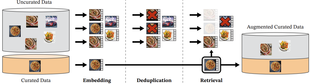
Diagram of curated images guiding retrieval from an embedded and deduplicated web-image pool
Figure 1. Construction of LVD-142M. Images in the gray uncurated pool are embedded and deduplicated. Images similar to examples from the orange curated sources are then retrieved and added to the curated collection.

The pipeline proceeds as follows:

The authors start with a raw web pool. URL filtering, near-duplicate removal, NSFW filtering, and blurring of identifiable faces reduce it to about 1.2 billion unique images.
They remove near-duplicates of the test and validation images used in the paper's benchmarks.
They assemble curated seed sources: ImageNet-22k, the ImageNet-1k training split, Google Landmarks, and several fine-grained datasets.
A self-supervised ViT-H/16 pretrained on ImageNet-22k embeds both pools. Cosine similarity and k-means then connect uncurated images to the curated sources.
For a sufficiently large query dataset, the pipeline retrieves four nearest neighbors per query. Smaller sources use cluster-based sampling with balancing limits.

Selection is driven by visual similarity rather than captions, hashtags, or class annotations. The curated seeds nevertheless shape the final distribution: they determine which regions of the 1.2-billion-image pool the retrieval process explores.

The paper reports that deduplication and retrieval used the Faiss similarity-search library on 20 nodes, each with eight V100-32GB GPUs, and took less than two days to produce LVD-142M.

Scaling the model and implementation🔗

The largest model is a ViT-g/14 with about 1.1 billion parameters. Training a teacher and student of that size adds memory, stability, and throughput constraints, so the implementation work is part of the method rather than an incidental detail:

Memory-efficient attention. The authors implemented a FlashAttention-style kernel (Dao et al., 2022). To suit GPU kernels, ViT-g uses an embedding dimension of 1536 with 24 heads, or 64 dimensions per head.
Sequence packing. Global crops at resolution 224 and local crops at resolution 98 produce sequences of different lengths. DINOv2 concatenates them and uses a block-diagonal attention mask, making the computation equivalent to separate forwards while improving efficiency. The low-level components are provided by Meta's xFormers library.
Efficient stochastic depth. Rather than calculate every residual branch and mask selected results, the implementation skips computation for dropped residuals. With the reported drop rate of 40%, this saves both compute and memory.
Fully Sharded Data Parallel. FSDP shards the student, teacher, and AdamW optimizer states across GPUs. Model shards remain in float32; backbone weight broadcasts and gradient reductions use float16, while projection-head gradients are reduced in float32 for stability.

On the same hardware, this implementation runs about $2\times$ faster than the iBOT implementation while using $1/3$ of the memory. Those figures compare these two implementations under the paper's setup.

Distilling the smaller models🔗

The authors train ViT-g/14 from scratch, then use it to teach the smaller ViT-S/14, ViT-B/14, and ViT-L/14 models. This is knowledge distillation: transfer the behavior of a large teacher into a cheaper student instead of repeating the complete pretraining recipe for every size.

For this stage, the teacher is fixed, masking and stochastic depth are removed, the iBOT loss is applied on the two global crops, and an exponential moving average of the student becomes the released model. In the paper's ablation, the distilled ViT-L/14 beats a ViT-L/14 trained from scratch across all 12 reported benchmarks.

How to read the experiments🔗

The paper evaluates classification, domain generalization, fine-grained recognition, video action recognition, instance retrieval, semantic segmentation, and monocular depth estimation. These results use three distinct protocols:

Non-parametric evaluation: compare frozen features directly, as in nearest-neighbor retrieval.
Linear evaluation: freeze the backbone and train a linear classifier on its output.
Dense prediction: freeze most or all of the backbone and train a decoder or adapter that converts patch features into segmentation or depth predictions.

This distinction matters because "frozen backbone" describes the encoder, not the entire downstream system. Architecture, pretraining data, input resolution, and readout capacity all belong beside a benchmark number.

Image classification🔗

With a frozen backbone and a trained linear classifier at resolution 224, DINOv2 ViT-g/14 reaches 86.5% ImageNet-1k top-1 accuracy. In the same evaluation table:

iBOT ViT-L/16 reaches 82.3%, so the reported improvement over the previous SSL result is 4.2 percentage points;
OpenCLIP ViT-G/14 reaches 86.2%; and
EVA-CLIP ViT-g/14 reaches 86.4%.

Under this linear-evaluation protocol, DINOv2 is competitive with and narrowly ahead of these weakly supervised baselines. Results vary by dataset, as the next transfer experiments show.

Supervised end-to-end fine-tuning raises ViT-g/14 from 86.5% to 88.5% at resolution 224 and from 86.7% to 88.9% at resolution 448. Frozen features provide a strong starting point; fine-tuning still adds 2.0 and 2.2 percentage points respectively.

Classification beyond ImageNet and video🔗

The paper trains linear classifiers on frozen DINOv2 features for iNaturalist, Places205, and 12 additional transfer datasets. DINOv2 is particularly strong on fine-grained categories, but OpenCLIP remains better on some benchmarks such as SUN and Stanford Cars.

For video action recognition, the frozen image encoder processes eight frames independently. The evaluation averages their features for UCF-101 and Kinetics-400, while Something-Something v2 concatenates them to preserve temporal order before training the linear classifier. The experiment tests whether frame-level visual features support action recognition; the pretraining objective itself remains image-based.

Instance retrieval🔗

Instance retrieval is the paper's direct, non-parametric use of the representation. The system computes one feature per image and ranks database images by cosine similarity to the query; there is no task-specific retrieval head. On Oxford-Hard, the strongest reported DINOv2 result improves by roughly 41 mAP points over the selected SSL baseline and 34 points over OpenCLIP.

The photograph on the right is the query. The numbered panels on the left are its ten highest-ranked database matches. The medium, color, pose, and background vary, yet every result depicts horses; several also retain the side-on pose or a multi-horse composition. The figure makes the behavior visible, while the Oxford-Hard score above provides the quantitative test.

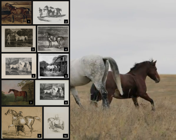
Query photograph of two horses beside ten ranked retrieved horse artworks
Figure 2. Instance-retrieval example. Right: a query photograph of a gray horse and a brown horse in a field. Left: ten retrieved horse images, ranked 1-10 by similarity in the frozen DINOv2 feature space. The matches span photographs, paintings, and line drawings while retaining the subject and some pose or composition cues.

Semantic segmentation🔗

Semantic segmentation assigns a class to every pixel. This directly tests whether the patch tokens preserve object boundaries and local category information. The paper keeps the backbone frozen and compares three increasingly capable predictors trained with semantic labels:

a linear layer on patch tokens;
a stronger multiscale linear setup using the last four transformer layers, a larger input, and multiscale inference; and
a trained ViT-Adapter plus Mask2Former head on top of the frozen backbone.

The multiscale ViT-g/14 setup reaches 53.0 mean intersection-over-union (mIoU) on ADE20K, close to MAE with end-to-end UperNet fine-tuning at 53.6. Adding the ViT-Adapter and Mask2Former raises DINOv2 to 60.2 mIoU while keeping 66% of the weights frozen; the cited state of the art reaches 62.9. The 7.2-point gain from the stronger readout measures how much more spatial information it can extract from the same frozen backbone.

Figure 3. Side-by-side qualitative comparison of segmentation outputs built from DINO and DINOv2 features. Cleaner boundaries and more stable regions make the improvement visible across frames. (Source)

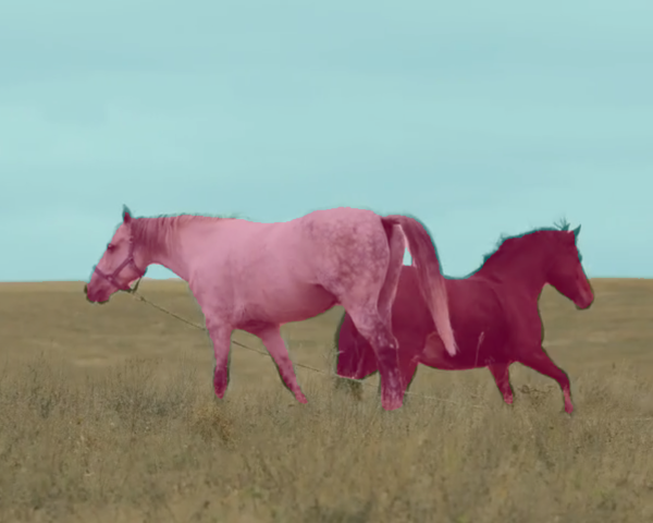
Semantic-segmentation overlay following two horses in a grassy field
Figure 4. A colored segmentation overlay follows the contours of both horses while leaving the field and sky as background. A task-specific predictor supplies the semantic output from frozen DINOv2 patch features.

Monocular depth estimation🔗

Monocular depth estimation predicts scene depth from a single image. The evaluation again freezes the DINOv2 backbone, then compares how much geometry three readouts can recover: a linear head over one transformer layer, a linear head over four layers, and a DPT decoder.

With DPT, DINOv2 ViT-g/14 reports root-mean-square error (RMSE) of 0.279 on NYU Depth v2, 2.11 on KITTI, and 0.338 when transferring from NYU Depth v2 to SUN RGB-D. Lower RMSE is better. The corresponding reference results in the paper are 0.330, 2.10, and 0.421: DINOv2 improves the NYU and transfer results and is effectively level with the KITTI reference.

Figure 5. Video examples pair input frames with color-coded depth predictions from a trained depth head operating on DINOv2 features.

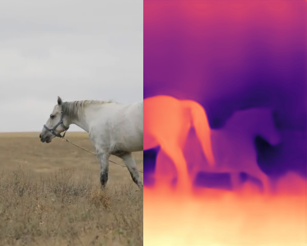
Photograph of a horse beside its color-coded monocular-depth prediction
Figure 6. Left: the input photograph. Right: the predicted relative-depth map, where the horse and nearby ground separate from the more distant scene. The depth head is trained; the DINOv2 backbone remains frozen.

Reading the patch-feature visualizations🔗

The paper uses principal component analysis (PCA) to turn high-dimensional patch features into a picture:

Compute PCA jointly over the patch tokens for each column of related images.
Threshold the first principal component to remove the background.
Map three subsequent components to red, green, and blue.

The colors are therefore coordinates in feature space, not class labels. When the same colors recur on the wings of different birds or the body of a horse in different styles, those patches vary along similar feature directions.

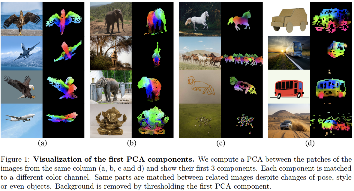
Related photographs and drawings paired with PCA-colored DINOv2 patch-feature maps
Figure 7. Each group pairs related source images with PCA-colored patch maps. Wings align across birds and aircraft, body regions align across elephants and horses, and vehicle parts align across drawings and photographs despite changes in pose, style, and category.

For explicit patch matching, the authors compute Euclidean distances between patch features from two images, solve an assignment problem, and retain salient matches with non-maximum suppression. Examples connect wings to wings, heads to heads, and functionally similar regions across photographs, drawings, poses, and even different objects.

Together, the PCA views and explicit matches show that local DINOv2 features encode useful correspondences across domains. Calling this "understanding object parts" is reasonable shorthand for the measured behavior: corresponding regions occupy corresponding locations in feature space. Symbolic or causal understanding would require a different experiment.

Applications and appropriate usage🔗

The experiments suggest a practical pattern: start with the frozen encoder, measure how far a simple readout gets, and add a stronger decoder or fine-tuning only when the task needs it. Suitable uses include:

image and video classification with a trained probe;
non-parametric instance retrieval;
semantic segmentation with a trained linear head or decoder;
monocular depth estimation with a trained head;
object detection and other dense tasks using adapters or decoders; and
specialized domains where labels or captions are scarce.

Cellular imaging is one plausible specialized domain because useful visual structure may be abundant while annotations are scarce. The paper presents this as an application direction rather than an evaluated result; it does not train a cellular foundation model or report a biological-discovery experiment.

Limitations, bias, and cost🔗

The paper reports five practical limitations:

Geographical and income bias remains. On Dollar Street, the ViT-g model has a 25.7-point performance gap between Africa and Europe and a 31.7-point gap between low- and high-income households. It improves on the selected SEERv2 baseline but remains biased toward wealthier households in Western regions.
The human-attribute analysis is limited. A linear classifier showed no clear harmful-label pattern across the evaluated gender, skin-tone, and age groups, but the authors explicitly state that a more thorough analysis could reveal additional flaws.
Training is expensive. Under the paper's standardized assumptions, reproducing one DINOv2-g run requires 22,016 A100 GPU-hours, about 9.7 MWh, and an estimated 3.7 tonnes of CO2 equivalent. The estimate covers GPU electricity and excludes hardware manufacturing and disposal.
Correspondence is narrower than general semantic reasoning. The PCA and patch-matching examples measure consistent local features; they do not test a general theory of object-part understanding.
The representation is not language-aligned. Image-only pretraining does not provide CLIP-style open-vocabulary labels. Applications that need named concepts must add a supervised or language-alignment component.

Future research🔗

The authors propose that object-part and scene-geometry properties may continue to improve with model and data scale, drawing an analogy to emergent abilities in language models (Wei et al., 2022). The current experiments motivate that hypothesis but do not trace a scaling curve for those properties.

They also suggest feeding frozen visual features into a language-enabled system as visual tokens. Such a system would need an additional alignment or multimodal training stage because the original DINOv2 representation is image-only.

Conclusions🔗

DINOv2's contribution is the complete recipe: DINO aligns image-level views, iBOT develops local patch features, KoLeo spreads global representations, LVD-142M supplies curated scale, and the implementation makes a 1.1-billion-parameter teacher trainable. Distillation transfers that representation into smaller models.

The experiments show where the work resides in a downstream system. The frozen backbone provides transferable image and patch features. Retrieval uses those features directly; classification, segmentation, and depth estimation add a trained readout, and full fine-tuning can improve them further.

References and resources🔗

The primary reference is "DINOv2: Learning Robust Visual Features without Supervision" by Maxime Oquab and colleagues. It was submitted to arXiv on 14 April 2023, revised in February 2024, and published in Transactions on Machine Learning Research (TMLR) in 2024. The OpenReview record contains the publication history, and the authors provide the official implementation and checkpoints.

DINOv2 builds on a line of self-supervised visual learning that includes DINO, iBOT, MAE, SEERv2, MSN, EsViT, and Mugs. Its weakly supervised comparison set includes CLIP, OpenCLIP, and SWAG.