Decision Transformer: Unifying sequence modelling and model-free, offline RL

The Decision Transformer paper explained.🔗

In this article we will explain and discuss the paper:

"Decision Transformer: Reinforcement Learning via Sequence Modeling": by Chen L. et al, ArXiv

that explores application of transformers to model sequential decision making problems - formalized as Reinforcement Learning (RL). By training a language model on a training dataset of random walk trajectories, it can figure out optimal trajectories by just conditioning on a large reward.

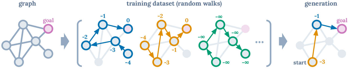Figure 1. Conditioned on a starting state and generating largest possible return at each node, Decision Transformer sequences optimal paths. (Source)

TL;DR🔗

• The idea is simple. 1) Each modality (return, state, or action) is passed into an embedding network (convolutional encoder for images, linear layer for continuous states). 2) embeddings are processed by an autoregressive transformer model, trained to predict the next action given the previous tokens using a linear output layer.
• Instead of training policy in a a RL way, authors aim at sequence modeling objective, with use of sequence modeling algorithm, based on Transformer (the Transformer is not crucial here and could be replaced by any other autoregressive sequence modeling algorithm such as LSTM)
• The algorithm is looking for actions conditioning based on the future (autoregressive) desired reward.
• Presented algorithm requires more work/memorizing/learn by the network to get the action for a given reward (two inputs: state and reward), comparing to classical RL where the action is the output based on the maximized reward for a policy. One input: state, to train the policy. However, authors tested how transformers can cope with this approach minding recent advancements in sequence modeling.
• Decision Transformer is based on offline RL to learn form historical sequence of (reward, state, action) tuples to output action, based on imitation of similar past reward and state inputs and action outputs.
• Solution is learning about sequence evolution in a training dataset by learning from agents' past behaviors for similar inputs: state and the presently required reward, to output an action.
• Limitation: If the credit assignment needs to happen longer than within one context. Thus, when relevant action for the reward is outside of the sequence that the Transformer attends to it will fail - as it would be out of the context.

Contribution of paper:🔗

• use the GPT architecture to autoregressively model trajectories
• bypass the need for bootstrapping (one of "deadly triad"¹) by applying transformer models on collected experience using sequence modeling objective
• enable to avoid discounting factor for future rewards used in TD thus, avoid inducing undesired short-range behaviors
• bridge sequence modeling and transformers with RL
• test if sequence modeling can perform policy optimization by evaluating Decision Transformer on offline RL benchmarks in Atari, OpenAI Gym, and Key-to-Door environments
• DecisionTransformer (without dynamic programming) match, or exceeds performance of SOTA model-free offline RL: Conservative Q-Learing (CQL), Random Ensemble Mixture (REM), Quantile Regression Deep Q-Network (QR-DQN) or behavioral cloning (BC)

Intro🔗

In contrast to supervised learning, where the agent that imitates actions will (by definition) learn at its best to be on pair with the input data (trainer), the Reinforcement Learning can learn how to be much better like in case of AlphaGo (Go), AlphaStar (StarCraft II), AlphaZero (Chess) or OpenAI Five (Dota2).

Transformer framework is known of its performance, scalability and simplicity, as well as its generic approach. The level of abstraction that is available via transformer framework reduces the inductive bias and thus, is more flexible and effective in multiple applications relying more on the data than on assumed, hand designed concepts. As this has already been proven in NLP with GPT and BERT models and Computer Vision with Vision Transformer (ViT), authors have adapted transformers to the realm of Reinforcement Learning (RL).

If you are already familiar with RL terms used in the intro you might want to go directly to the Decision Transformer paper motivation explained. For more explanation of the terms referred in the paper please see prerequisite RL knowledge section.

Motivation🔗

Transformer framework has proven to be very efficient in multiple applications in NLP and CV by modeling high-dimensional distributions of semantic concepts at scale. Due to natural consequence of transformer nature, the input should be in form of a sequence thus, in case of Decision Transformer the RL has been casted as conditional sequence modeling. Specifically, the sequence modeling (with transformers) for policy optimization in RL is adapted by the Decision Transformer as a strong algorithmic paradigm.

One very interesting motivation for using transformers is that they can perform credit assignment directly via self-attention, in contrast to Bellman backups which slowly propagate rewards and are prone to “distractor” signals. This might help transformers to work with sparse, or distracting rewards. It even made Decision Transformer (DT) to outperform RL baseline for tasks requiring long term credit assignment due to the usage of long contexts. The DT aims to avoid any inductive bias for credit assignment, e.g. by explicitly learning the reward function or a critic, in favor of natural emergence of such properties thanks to transformer approach.

Objective, or goal for the algorithm🔗

The goal is to investigate if generative trajectory modeling – i.e. modeling the joint distribution of the sequence of states, actions, and rewards – can serve as a replacement for conventional RL algorithms.

The processing strategy of the algorithm🔗

The classic RL is focused on maximizing the reward for a state, by finding an action that actually will maximize the reward. Conversely, the key aspect of DT is to condition on future desired reward. Consequently, algorithm has additional - reward - input, along with the state. This way it is expected not only to maximize, but to fit to the actual reward value. That however, requires more learning/memorization. This is where transformers have proven to work particularly well for sequence modeling. Natural consequence of this design decision is to use the offline RL. This is why the paper is focused on the world of model-free and offline RL algorithms.

The tasks expects to find the right action for a given state and reward. The offline nature allows the Transformer to look into historical (offline, training dataset) data to find the same state with similar history and about the same reward for future action. From such past experience, similar action will be deduced ²

Figure 2. Decision Transformer overview (Source).

the Transformer outputs an action that agents (in the past) ended up with, for same state, while getting similar reward. Such action is what agent is expected to get in current timestep. (See Figure 2.).

The major drawback of this approach is that it is limited to the context sequence length. Thus, in case when agent commenced action more aligned for current state-reward condition, but which is outside of the context (self-attended input of Transformer) - the sequence model will not be able to infer about that, as it only attends to tokens within the limited length context.

Therefore, the DT is better for credit assignment for longer distances than the LSTMs (see more), but the drawback is that it still does not allow to ditch the classical RL dynamic programming methods, as the are still suitable for the longer-than-context learning problems.

Another important aspect to note is that with minimal modifications to transformer, DT models trajectories autoregressively. The goal here is to be able to conditionally generate actions at test time, based on future desired returns $\hat{R}$ (using modeled rewards) rather than past rewards.

A trajectory - $\tau$ - is made of sequence of states, actions and rewards at given timesteps: $\tau = (s_0, a_0. r_0, s_1, a_1, r_1, \ldots, s_T, a_T, r_T)$ The return of a trajectory at $t$ timestep, is the sum of future rewards of the trajectory starting from $t$: $R_t = \sum_{t'=t}^T r_{t'}$ (without discount factor³).

The goal of offline RL is to learn a policy which maximizes the expected return $\mathbb{E}[\sum_{t=1}^T r_t]$ in an Markov Decision Process (MDP). However, the DT instead of feeding rewards $R$ directly, uses (future) returns-to-go $\hat{R}$. Therefore, the trajectory becomes: $\tau = (\hat{R}_1, s_1, a_1. \hat{R}_2, s_2, a_2, \ldots, \hat{R}_T, s_T, a_T)$. After executing the generated action for the current state, algorithm decrement the target return by the achieved reward and repeat until episode termination.

The input of the architecture is a state that is encoded with DQN encoder with linear layer to project to the embedding dimension followed by layer normalization. To obtain token embeddings, a linear layer is learned for each modality (return-to-go, state, or action), which projects raw inputs to the embedding dimension. The linear layer is replaced with convolution encoder for environments with visual inputs. An embedding for each timestep is learned and added to each token – this is different from the standard positional embedding used by transformers, as one timestep corresponds to three tokens (one for each modality: return-to-go, state, or action). The tokens are then processed by a GPT model, which predicts future action tokens via autoregressive modeling.

The training use a dataset of offline trajectories. Samples minibatches of sequence length K are used from dataset. TThe prediction head corresponding to the input token $s_t$ is trained to predict $a_t$ either with cross-entropy for discrete actions, or mean-squared for continuous actions while the loses are averaged.

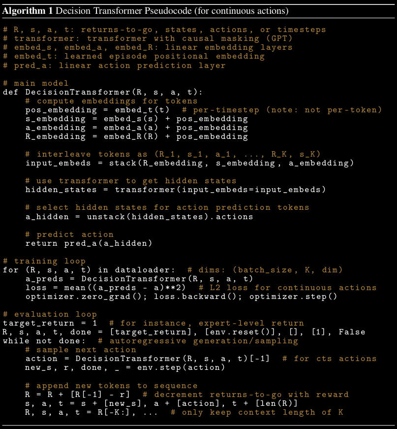Figure 3. Decision Transformer Pseudocode (Source).

Metaphors, or analogies to other architectures describing the behavior of the algorithm🔗

There are two main approaches for offline learning that are compared to Decision Transformer: Behavioral Cloning (BC) and Conservative Q-Learning (CQL). The BC is to simply mimic behavior in episodes that has lead to good rewards.

CQL limits the tendency of Q-functions in the offline setting to overestimate the Q-value that results from certain actions.

The considerations of the DT🔗

An important aspect that should be mentioned about DT is related to its offline learning nature. That is, the high dependency on the dataset that is picked as the training set of episodes. In the paper, the dataset is based on experience of DQN high performing agent, as an active reinforcement learner. This way the source episodes in dataset are not a random demonstrations, but are more of a set of expert demonstrations.

Additionally, DT is a sequence model and not an RL model. Interestingly, the transformer part of DT, could be replaced with any other autoregressive sequence modeling architecture such as LSTM. In which case the past (state, action, reward) tuples can get propagated as a hidden representation, one step at a time, while producing next action (or a Q-value in case of Q-learning) that results with a certain reward.

The LSTMs finds the decisive action that lead to the expected result (during training) in a sequence of actions. As we are looking for this most meaningful actions to gain the expected final state, it is not the last action in the sequence of state changing actions, that might be the best. The goal of RL is to assign the highest reward to this most meaningful action in an episode. This way in future this actions will be favored.

For LSTMs this requires to go back though the episode sequence of states (and actions) deeper with Back Propagation Though Time (BPTT)⁴ which limits how far back the error is propagated (to at most the length of the trajectory) because it is computationally expensive, as the number of timesteps increase in LSTM (as a RNN variant).

Therefore, it is a very hard (esp. in architectures like RNN/LSTM) task to do the long-range time credit assignments.

To solve this problem a dynamic programming is used in RL. Therefore, instead of having to just learn from the reward and assign it to an action, each timestep will output not only an action, but also a value (similarly as Q-function already returns a value in Q-learning). The algorithm that does this is called Temporal Difference learning.

The value is the expected/estimated return (final reward in the future) of the episode, starting from the given state, and following till the final state (return) is reached. This way, the final return prediction is not the only learning signal, but also this gives predictions of future reward values for the next actions in each of the intermediate, consecutive states in the path that leads to the final return state. In other words, at each state the value function not only tries to predict the final return (which is really noisy for states that are far from return), but also train the value function to predict all the values from states that are between the current state and the final one in an episode. Thus, trying to predict the output of the value function.

Bellman (aka backup / update) operator - operation of updating the value of state $s$ from the value of other states that could be potentially reached from state $s$.

Bellman equation for the V-function (State-Value) simplifies computation:

\begin{equation} v^\pi (s)= \mathbb{E_\pi}[R_{t+1} + \gamma v(S_{t+1})| S_t = s] \end{equation}

Bellman equation decomposes the V-function into two parts, the immediate reward - $R_{t+1}$ - plus the discounted future values of successor states. This equation simplifies the computation of the value function. This way, rather than summing over multiple time steps, we find the optimal solution of a complex problem by breaking it down into simpler, recursive subproblems and utilizing the fact that finding their optimal solution to the overall problem depends upon the optimal solution to its subproblems. Which make it a dynamic programming algorithm similarly to the Temporal Difference approach,

It works similarly in terms of the Q-function (State-Action value function) in Q-learning, where this approach is formalized with the Bellman's recurrence equation.

\begin{equation} q_\pi (s,a) = \mathbb{E_\pi}[R_{t+1} + \gamma q_\pi (S_{t+1}, A_{t+1})| S_t=s, A_t=a] \end{equation}

Here, State-Action Value of a state can be decomposed into the immediate reward we get on performing a certain action in state $s$ and moving to another state $s_{t+1}$, plus the discounted value of the state-action value of the state $s_{t+1}$ with respect to the some action $a$ our agent will take from that state on-wards.

In RL we use the TD learning and Q-functions to allow credit assignment for long time ranges.

However, as the DT is a sequence modeling problem there is no need for dynamic programming techniques such as Temporal Difference (TD) to be applied. This is due to the Transformer nature, that enables to attend (route information) from any sequence element to any other sequence element in a single step. Therefore, technically the credit assignment can be done in a single step - but under one crucial condition: as as long as if it fits into context.

Limitations🔗

The limitation of this credit assignment approach is that this works only for a given length of Transformer input sequence (context). If one would like to predict correlations and do the credit assignment across longer spans, than the Transformer input sequence (as a context), still the dynamic programming would be required.

Heuristics or rules of thumb🔗

The DT has been tested on the Atari dataset. The Figure 4. show that DT outperformed remaining algorithms on most of the games however, with high standard deviation.

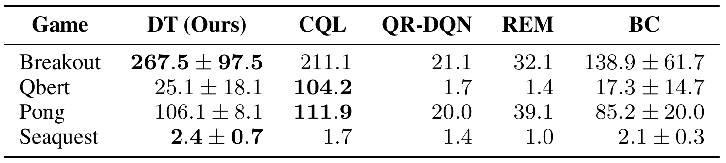Figure 4. Decision Transformer Pseudocode (Source).

The lower standard deviation and also mostly better results, comparing to CQL, are presented for OpenAI Gym considering the continuous control tasks from the D4RL benchmark.

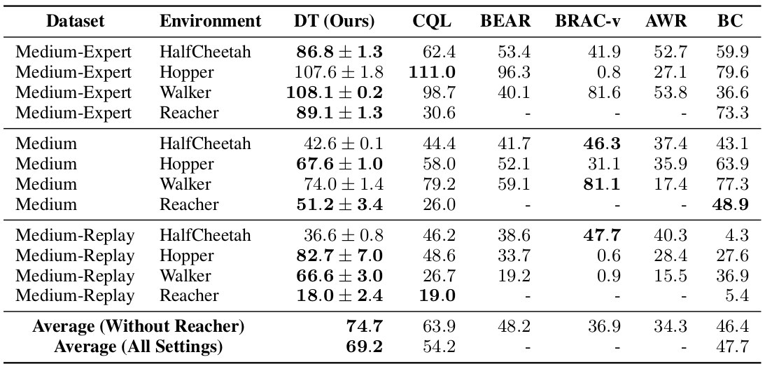Figure 5. Decision Transformer (DT) outperforms conventional RL algorithms on almost all tasks. (Source).

Additionally, comparing to behavioral (see Figure 6.) cloning trained on set percent of the experience 10, 25, 40, 100 percent. The results show that BC can give better performance than DT if the choice will select certain percentage not necessarily picking the best trajectories. To find the right percentage additional hyper-parameter search i requires, while DT is just one run solution.

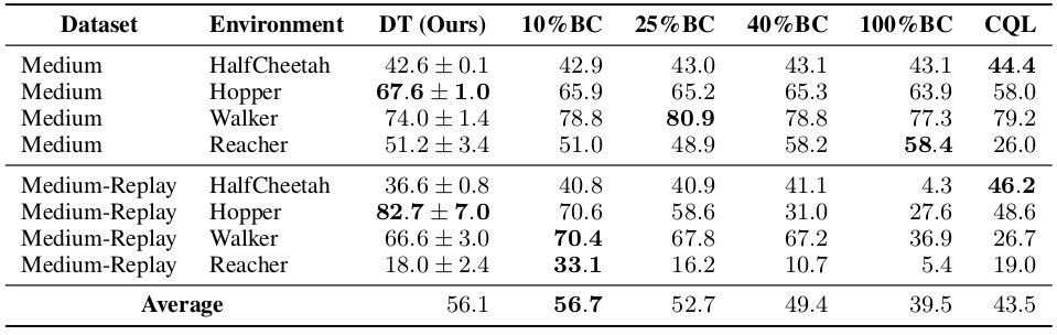Figure 6. Comparison between Decision Transformer (DT) and Percentile Behavior Cloning (%BC). (Source).

However, one should note that in each of the experiments the DT hyperparameters are different. For instance, whenever a task is a sparse reward task, the context length is increased to limit the impact of the context boundary limitation as described in previous sections. To confirm this Table 5 in the paper shows that the longer the context the better performance DT achieves.

Additionally, in experiments such as the game of Pong, where the reward is known to be at max 21, this fact has been used to condition on the reward of 20 (see Table 8 of the appendix). Therefore, the fact of knowing the reward seems very important to setup the hperparameters correctly for DT.

The limitation of DT seems to be that you need to know the reward that task is aiming for and according to Figure 4. of the paper putting arbitrary large value for reward is not possible. From that graph, when the green line of expected oracle is aligned with the blue line of the DT outcome, this means that the reward is as expected. However, soon after the received reward is higher than the one observed from the training dataset performance drops.

Key-to-Door🔗

One final example is the Key-to-Door environment, where the use of Transformer with longer context is proving being appropriate for long-term credit assignment. This however is only limited to the size/length of the context. Interestingly, authors have used entire episode length as the context.

The process has three phases:

• agent is placed in a room with a key
• agent is placed in an empty room ("distractor" room to allow to forget the information from the first room)
• agent is placed in a room with a door

The agent receives a binary reward when reaching the door in the third phase, but only if it picked up the key in the first phase. This problem is difficult for credit assignment because credit must be propagated from the beginning to the end of the episode, skipping over actions taken in the middle.

The Figure 7. shows that with the DT, if the agent does not pick up the key in the first room, it already knows in second room that the game is lost due to being within the context of Transformer's attention. This knowledge is from the past offline episodes where not picking the key means that the game is lost.

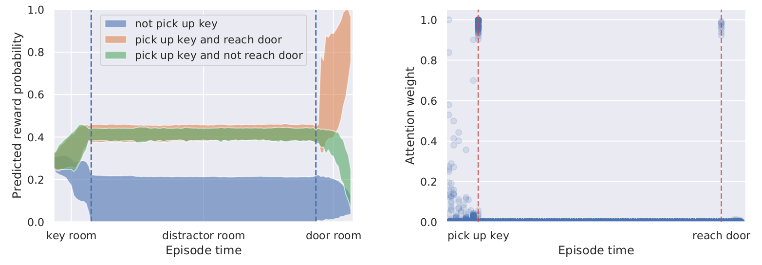Figure 7. Comparison between Decision Transformer (DT) and Percentile Behavior Cloning (%BC). (Source).

What classes of problem is the algorithm well ?🔗

According to the test results, as long as the context length of the Decision Transformer matches the task expectation, the solutions behaves better than other methods like CQL or BC. However, to achieve this, one needs to know the length of the context in form of a hyperparameter.

Additionally, for the sake of the performance, knowing the maximum reward is also important.

Common benchmark or example datasets used to demonstrate the algorithm🔗

Decision Transformer can match the performance of well-studied and specialized TD learning algorithms developed for these settings.

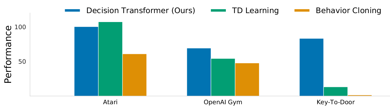Figure 8. Results comparin DT to TD learning (CQL) and behavior cloning across Atari, OpenAI Gym, and Minigrid. (Source).

As DT is based on a offline mode, a very important part of offline RL is how do we pick this fixed dataset to model upon. Here it is based on DQN expert learner, so the results are good and far from being random.

In the paper authors compare DT to two approaches that are used in offline RL setup:

• Behavioral Cloning (BC) where the agent tries to mimic those agents from the dataset, which have gained high rewards for their actions.
• Q-Learning (actually a Conservative Q-Learning) (CQL). Q-learning is a classic RL algorithm which uses Q-function to estimate Q-values, along the possible state and action space, to maximize the total reward. The Conservative Q-learning (CQL) is more of a pessimistic approach, that helps to mitigate the tendency of Q-function to overestimate the Q-values that one gets from certain actions.

Useful resources for learning more about the algorithm:🔗

• ArXiv Paper
• GitHub implementation

---

Footnotes:🔗

1. When one tries to combine time difference (TD) learning (or Bootstrapping), off-policy learning, and function approximations (such as Deep Neural Network), instabilities and divergence may arise. ↩
2. Similarly to behavioral cloning which maximizes the reward based on expert demonstrations.[\ref]. This way based on the past sequence experiences, ↩
3. The discount factor $\gamma$ presence (in eg CQL) in the return calculation is a design decision for the problem formulation and it enables stability of the solution at price of discounting more of the future distant rewards than the closer ones in an episode. ↩
4. one trains recurrent neural networks by unrolling the network into a virtual feed forward network, and applying the backpropagation algorithm to that. This method is called Back-Propagation-Through-Time (BPTT), as it requires propagation of gradients backwards in time. ↩