MLP-Mixer: MLP is all you need... again? ...

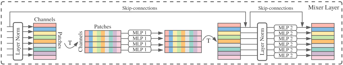
TL:DR🔗

MLP is all you need to get adequately comparable results to SOTA CNNs and Transformer - while reaching linear complexity in number of input pixels. Conversely to CNNs, MLP is not localized as its filter spans entire spatial area

The return to this idea deserves some deeper consideration. If you start thinking that researchers have already been here please read:

(...) As in the games, researchers always tried to make systems that worked the way the researchers thought their own minds worked---they tried to put that knowledge in their systems---but it proved ultimately counterproductive, and a colossal waste of researcher's time (...)

The Bitter Lesson form Rich Sutton, March 13. 2019

Contribution of paper:🔗

• Proves that MLP based architecture can be on pair with modern SOTA in terms of accuracy and computational resource trade-off for training and inference.
• Mixer has linear computation complexity in number of input pixels, in contrast to ViT and similarly to CNNs.
• Unlike ViT, no need for position embedding (token-mixing MLP is sensitive to the order of input tokens)
• Uses standard classification head with global average pooling followed by linear classifier.
• Mixer-MLP scales better than attention based counterparts for bigger training sets to an extend that it is on pair with them¹.

Raise questions on:

• How useful would it be to compare the features learned from CNN/Transformer solutions and those learned from such a simple architecture?

Consequently:

• What is the role of the inductive biases of such features and how they influence the generalization?

Intro🔗

In this article we will investigate the paper:

"MLP-Mixer: An all-MLP Architecture for Vision" Ilya Tolstikhin et al. 2021: ArXiv - Submitted on 4 May 2021

The current, established computer vision architectures are based on CNNs and attention. The self-attention oriented modern Vision Transformer (ViT) models relies heavily on learning from raw data. The idea presented in the paper is simply to apply MLP repeatedly for spacial locations and feature channels.

Motivation🔗

The Transformer/CNN trend in the area has dominated research in terms of SOTA results. Authors claim that the paper goal is to initiate discussion and opening questions on how the feature learned from both the MLP and present dominating approaches can be compared? It is also interesting how the induced biases contained within the features compares and influence the ability to generalize.

The processing strategy of the algorithm🔗

Similarly to the Vision Transformer. Each input image is divided into a grid of linearly projected, non-overlapping $16\times 16$ pixel patches (tokens). Patches are put into one table of $patches\times channels$ as an input for the architecture. This is conversely to previous architectures, where patches would be unrolled into one, single vector of consecutive patches.

The patches are basic parts that the architecture is working on as they are propagated through the network. The Mixer stacked layers are all of the same size. This is unlike CNNs where we shrink the resolution, but increase the channels.

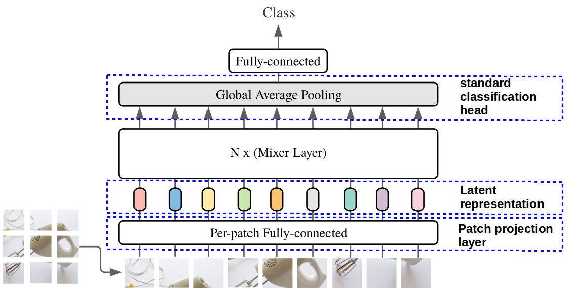
Figure 1. MLP-Mixer general architecture.

At first every patch is feed through per-patch, fully connected layer, providing the latent vector representation (embeddings) per each patch. This is then passed to multiple Mixer layers of the same size – each layer build out of two MLP blocks.

There are two types of Mixer-MLP blocks that acts on rows and columns of the input table:

1. Token-Mixing ; $Channels \times Patches$ (acts on columns) enables communication across different spacial locations (tokens) of an image present in a single channel. A single column of the input table collects all tokens’ parts (across different patches) of a single channel.

2. Channel-Mixing $Patches \times Channels$ (acts on rows); enables communication across different channels as their input is an individual token as a row from the input table.

MLP-Mixer use the idea of small kernel convolutions. The channel-mixing MLP_2 with $1\times1$ convolutions becomes effectively dense matrix multiplication applied independently to each spacial location. However, it does not allow aggregation of cross-spacial information. This motivates the token-mixing MLP_1 phase that includes the dense matrix multiplications applied to each feature/channel across all spatial locations.

The MLP block structure🔗

The latent representation of patches form the fully-connected layer is first feed into the token-mixer in a $channel x patch$ table. Whit that in mind, it takes all the patches (columns) per channel (row) and feeds it to the MLP1 (two fully connected layers connected with GELU). Each MLP consists of two fully-connected layers and a non-linearity - GELU - applied independently to each row of its input data tensor.

The Mixer approach, is based on the idea that channels in individual patches mean similar things. It is because they come from same function of the per-patch fully-connected layer. This first layer put same object information into same channels for different patches. Thus, as they mean similar things, we will group them by channels, and aggregate over all patches within each channel. Therefore each channel have same information in form of feature.

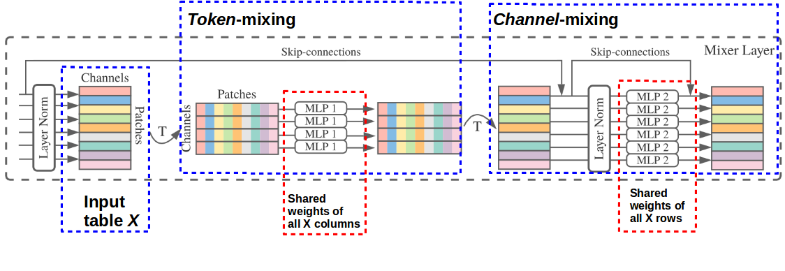
Figure 2. Detailed architecture schema of MLP-Mixer layer.

Each of the patches is feed through the same MLP1 with shared weights across all columns of the input table. Thus, we are dealing here with a dense matrix multiplication with a weight sharing across same channel of different patches². In token-mixing, the MLP_1 share the same kernel (of full receptive field) for all of the channels. Therefore, if a channel reacts as a feature across the patches, it is easy to aggregate all the patches that include this feature.

Second stage is to transpose back to $patches x channels$ and repeat same computation in MLP_2 however, this time with weight sharing across all patches (rows of the input table). This kind of sharing provides positional invariance, which happens to also be part of CNNs. For each patch we apply computation across all of the channels (features) of that patch.

Other components include: skip-connections, dropout, layer norm on the channels, and linear classifier head

Objective or goal for the algorithm🔗

The general idea of the MLP-Mixer is to separate the channel-mixing (per-location) operations and the cross-location (token-mixing) operations. This is what distinguish it from the solutions described in following section. This way if we aggregate among the same channels (token-mixing) then if a channel reacts across the patches we can aggregate all the patches that have that feature because the feature producing map was shared.

Mixer computational complexity is linear in the number of input patches (input sequence length) in token-mixing, conversely to the previous ViT architecture - whose computational complexity is quadratic. Additionally, as the channel hidden width in channel-mixing, is also independent of the patch size, the overall complexity is linear in the number of pixels. Which is also the case with CNNs.

Metaphors, or analogies to other architectures describing the behavior of the algorithm🔗

The MLP-Mixer does not use the convolutions, nor self-attention - which are heavily used by the current successful architectures.

Reference to remaining, modern vision architectures can be based on two techniques of layers that mix features at:

1. one spatial location
2. across different spatial locations,

Both of those can be applied exclusively, or at once.

In CNNs - deeper layers have larger receptive field – with $N \times N, N>1$ convolutions and pooling implement the second approach while with $1 \times 1$ would use first one.
The Mixer architecture is a very special case of CNN with $1 \times 1$ convolutions in channel-mixing, and for token-mixing it is a single-channel depth-wise convolution of a full receptive field with parameter sharing. Conversely, CNNs are not special cases of MLP-Mixer as the plain matrix multiplication of Mixer is less complex than costly convolutions specialized implementation.

While referring to the attention-based architectures such as Vision Transformers, the self-attention enables both techniques while the MLP blocks are focusing only on the first one.

The Mixer architecture embrace both techniques (using MLPs), but separates them clearly: the first, per-location operations is implemented in channel-mixing, and the cross-location operations are implemented with the token-mixing

Similarly to Transformers, each layer in Mixer (except for the initial patch projection layer) takes an input of the same (aka isotropic) size. This is in contrast to typical CNN that have a pyramidal structure: deeper layers have a lower resolution input, but more channels³.

Discussion: Is MLP-Mixer a simple a CNN only with the convolution weights being decided by attention?🔗

One can argue that this is simply a convolution in form of the "image patches" and that due to that the only thing that is proven here is that: the larger the receptive field is - the better results we can get. In which case this would be simply a $16\times16$ non-overlapping filters (stride 16). Moreover, then the architecture would be simply an MLP over kernel

However, if we take a closer look, the CNN is localized, so as such the filter is not covering the whole spacial area, with the Mixer it does.

Heuristics or rules of thumb🔗

Authors have commenced series of tests with couple of parameters. The patch resolution e.g. $16 \times 16$. The scale expressed in number of mixer layers: Small: 8, Big: 16, Large: 24 and Huge: 32 following the Vision Transformer (ViT) paper approach⁴.

The results of the experiments shows that the MLP-Mixer is comparable with current SOTA however, is not as good. Therefore, authors have found a metric that distinguish the Mixer architecture. It is the Throughput (column 5 in the below figure) defined as number of images per second per computation core.

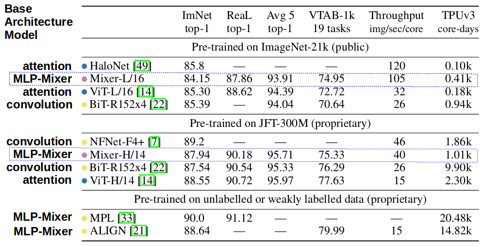
Figure 3. Transfer performance, inference throughput, and training cost.Sorted by inference throughput.

Additionally, authors have found out that on a very particular task of training linear 5-shoot classifier on frozen representation of what the model outcomes evaluated on Top-1 accuracy.

Note: Top-1 accuracy is the conventional accuracy, model prediction (the one with the highest probability) must be exactly the expected answer. It measures the proportion of examples for which the predicted label matches the single target label.

This has been evaluated, and discussed in context of the role of model scale.

Scalability - Mixer is catching up🔗

With training set size increase the authors state that the scalability of Mixer is much more favorably comparing to big transfer (BiT) that plateaus and is on pair with ViT. Moreover, in all cases the differences in the scalability performance of Mixer is getting very close, if not same, as remaining models.

Figure 4. Transfer performance, inference throughput, and training cost.Sorted by inference throughput.

This is the most significant result, but authors compare also some more tasks, for details please refer to the paper. The conclusion from the results however might be, that the smaller the training set, the worse the Mixer performs in terms of pre-training, and the bigger training set, the gap between the Mixer and remaining architectures (ViT, BiT) shrinks.

Weight visualization🔗

The weight visualization analysis confirm the general assumption on how we observe the neural network work. In the image we see that lower layers learn first the most general features (left), then go to bit larger ones (middle) and the detailed (right).

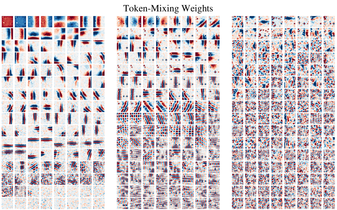
Figure 5. MLP-Mixer input weights to hidden units visualization in token-mixing MLPs of Mixer-B/16 model trained on JFT-300M proprietary Google dataset used for training image classification models.

Interestingly the weights visualization differs based on the type of the training set that authors have used:

What classes of problem is the algorithm well suited?🔗

The architecture seems useful especially for big scale training sets of vision tasks - as tested according to the description in next section. However, it might as well be applied to some NLP tasks however, with adequately prepared text “patches”.

Common benchmark or example datasets used to demonstrate the algorithm🔗

Comparing to CNN or attention based is claimed to be on pair with the existing SOTA methods in terms of the trade-off between accuracy and computational resources required for training and inference. Authors have tested downstream tasks such as:

• ILSVRC2012 “ImageNet” (1.3M training examples, 1k classes) with the original validation labels and cleaned-up ReaL labels,
• CIFAR-10/100 (50k examples, 10/100 classes),
• Oxford-IIIT Pets (3.7k examples, 36 classes), and
• Oxford Flowers-102 (2k examples, 102 classes) and also evaluate on the
• Visual Task Adaptation Benchmark (VTAB-1k), which consists of 19 diverse datasets, each with 1k training examples.

Footnotes:🔗

1. One interesting question is what would happen with even bigger training sets than the ones used in experiments? Would Mixer supersede remaining SOTA architectures? ↩
2. Tying parameters across channels is less common with contrast to previous solutions based on CNNs and self-attention. ↩
3. One can also refer to one of the non-typical designs, of other combinations such as isotropic ResNets and pyramidal ViTs. ↩
4. One of the authors has actually also coauthored that ViT paper. ↩