Neural Networks Primer

If any of the topic will grow enough I will put it into a separate post. To get in-depth understanding I recommend for:

• NLP: the Yoav Goldberg's, 2016 A Primer on Neural Network Models for Natural Language Processing

RNN primer with Gradient Descent (GD)🔗

Convolutional Neural Networks (CNN)🔗

Activation Functions🔗

There are two types of activation functions: saturating and non-saturating. Saturating means that such function squeezes the input.

• I.e. $f$ is non-saturating ⇔$(|\lim_{z\rightarrow−\infty}f(z)|=+\infty)\lor|\lim_{z\rightarrow+\infty}f(z)|=+\infty)$,
• and if $f$ is NOT non-saturating then it is saturating

phew! :)

Useful article and ReLu vs Softmax. Also part of cs231n

Recurrent Neural Networks(RNN) Vs Feedforward Neural Nets (FNN)🔗

RNN bring much improvement over FNN due to provided internal representation of past events (a.k.a. memory). RNN-based deep learning was so successful in sequence-to-sequence (s2s) due to its capability to handle sequences well. It should be noted that RNNs are Turing-Complete (H.T. Siegelmann, 1995)), and therefore have the capacity to simulate arbitrary procedures.

If training vanilla neural nets is optimization over functions, training recurrent nets is optimization over programs.

RNN is thus also able to learn any measurable s2s mapping to arbitrary accuracy (B.Hammer, 2000, On the Approximation Capability of Recurrent Neural Networks). So we get great results in handwriting recognition, text generation and language modeling (Sutskever, 2014). The availability of information on past events is very important in RNN. The problem however arise, in case when lacking prior knowledge on how long the output sequence will be. It is because the training targets have to be pre-aligned with inputs and standard RNN simply maps input to output. Additionally it is not taking into account the information from past outputs. One solution is to employ structured prediction where two RNN can be used to: model input-output dependencies (transcription) and second to model output-output dependencies (prediction). This way each output depends on entire input sequence and all past outputs.

Another limitation of RNN is the size of internal state. It can be seen on an example of encoder-decoder architecture for Neural Machine Translation (NMT). Here the encoder gets entire input sequence word by word while updating its internal state. While the decoder decodes it into e.g. other language.

Encoder-Decoder scheme🔗

Seq2seq modeling is a synonym of recurrent neural network based encoder-decoder architectures (Sutskever et al., 2014; and Bahdanau et al., 2014). Let us “unroll” the scheme into $M$ encoder steps and $N$ decoder steps of hidden states $h$.

Figure 1. Encoder-decoder architecture – example of a general approach for NMT. An encoder converts a source sentence into a "meaning" vector which is passed through a decoder to produce a translation.

In encode-decoder architecture¹, the

• encoder – maps input data $x$ to a different (lower dimensional, compressed – i.e. encoded) representation, while the
• decoder – maps encoder’s output new feature representation back into the input data space as a output sequence $y$; left to right one at a time. Decoder generates $y_{i+1}$ token by computing new hidden state $h_{i+1}$ based on:
  • previous hidden $h_i$ state
  • an embedding $g_i$ of the previous target language word $y_i$
• conditional input $c_i$ derived form the encoder output - $z$.

$$input:(x_1, \dots, x_m) \xrightarrow[\text{maps}]{\text{encoder}} z=(z_1,\dots,z_m)\xrightarrow[\text{generates}]{\text{decoder}} output: (y_1,\dots, yn)$$

One can consider two types of models, with or, without “attention”. The latter assumes $\forall i c_i=z_m$ (Cho et al., 2014)

Additionally, there is a problem with the encoder’s state $h^{E}_m$, as a compressed and fixed-length vector. It must contain whole information on the source sentence. This looses some information². One can try to use some heuristics that can help to overcome this issue and improve performance of RNN:

• Organize input. Feed the input more than one time or provide input followed by reversed input ³.

• Provide more memory. It turns out that the bigger the size of the memory the better (eg. LSTM applied to language modeling⁴) the RNN performs on various tasks.

To avoid the memorization problem there has been research on the attention mechanism.

Attention basis🔗

The most intuitive attention definition I know is the one contained within paper about Transformer architecture:

An attention function can be described as mapping a query and a set of key-value pairs to an output, where the query, keys, values, and output are all vectors. The output is computed as a weighted sum of the values, where the weight assigned to each value is computed by a compatibility function of the query with the corresponding key.

We will try to formalize this (let me know your suggestions) in the following form:

$$\begin{eqnarray} A(q, {(k,v)} ) \xrightarrow[\text{output}]{\text{maps as}} \sum_{i=1}^k{\overbrace{f_c(q,k_i)}^{\theta_i}}v_i, q \in Q, k \in K, v \in V \end{eqnarray}$$ $$Q, K, V – vector space, f_c- compatibility function$$

Concretely, an attention mechanism is distribution of weights over the input states. It takes any number of inputs ${x_1, ..., x_k}$, and a query $q$, and then produces weights ${\theta_1, ..., \theta_k}$ for each input. This measures how much each input interacts with (or answers) the query. The output of the attention mechanism, $out$, is therefore the weighted average of its inputs: $$ \begin{eqnarray} out = \sum_{i=1}^k \theta_i x_i \end{eqnarray}$$

Hence, networks that use attention, attend only on a part of the input sequence while still providing the output sentence. So one can image it as giving an auxiliary input for the network in form of linear combination. What is the clue here is that the weights of the linear combination are controlled by the network. It has been tested across multiple areas such as NMT or speech recognition.

In an encoder-decoder architecture for the embedding (fixed size vector) of a long sentence brings the problem of long dependency (e.g. in fixed-size encoded vector $h^E_N$, where end word of the sentence depends on the starting word $h^E_1$). And long dependencies, is where RNN have problems. Even though “hacks” such as reverse/double feeding of the source sentence, or the LSTMs (memory), are sometimes improving the performance however, they do not always work perfectly⁵. It is because the state and the gradient in LSTM would start to make the gradient vanish. It is called “long” time memory but its not that long to work e.g. for 2000 words. This is where convolutions came in.

Figure 2. WaveNet (left; sound) (image courtesy) and ByteNet (right; NLP) architecture (Image acquired from Neural Machine Translation in Linear Time, Kalchbrenner et. al 2016).

This is why the fixed size encoding might be a bottleneck of performance. This is where the attention comes in.

Attention is used as an alternative to memorizing and input manipulations. Here the model search for parts of a source sentence (not fixed size vector) that are relevant to predicting a target word, and it should attend to, based on what it has learned in the past Bahdanu et al., 2016.

Figure 2. Attention architecture.

In this case, the larger $\theta_{1,2}$ would be the more decoder pays attention for the $y_3$ (third output word) in relation to other words as all weights ($\theta$s) are normalized to sum to $1$.

Figure 3. “Attention”; the blue link transparency represents how much the decoder pays attention to an encoded word. Less transparent, more attention. Google Blog also general-purpose encoder-decoder framework for Tensorflow

It is well visualized in an $\theta$ matrix for French-English translation (See Figure Adopted form Bahdanu et al., 2016)

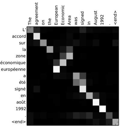
Figure 4. Attention matrix. Adopted form Bahdanu et al., 2016)

In French input sentence two words “la zone” are especially target for attention when translating to English “Area”.

This matrix of size InputSize $\times$ OutputSize is filled by calculating attention for each output symbol toward over every input symbol. This gives us $#Input^{#Output}$. For a longer sequences it might grow intensively. This approach requires a complete look-up over all input output elements, which is not actually working as an biological attention would. Intuitively attention should discard irrelevant objects without the need to interacting with them. What is called “attention” therefore is simply a kind of memory that is available for decoder while producing every single output element. It does not need the fixed-size encoded vector of the entire input. The weights only decide which symbols/words to get from the input-memory of the encoder. This so called attention is the subject of further development in form of End-To-End Memory Networks where recurrent attention is used where where multiple computational steps (hops) are performed per output symbol. This includes reading the same sequence many times before generating output and also changing the memory content at each step.

We can of course employ backpropagation to accustom the weights in an end-to-end learning model.

Layer connections 🔗

In Deep Learning networks architectures the problem of vanishing gradient is very common issue. Thus, some methods has been develop to mitigate its influence on the networks’ efficiency.

Highway layers🔗

Residual connections🔗

Models with many layers often rely on shortcut or residual connections (Zhou et al., 2016; Wu et al., 2016). This trick has become main factor for He et al. 2016 CVPR winning the ImageNet 2016 Residual connection is a connection between layers that adds the input $x$ of the current layer to its output via a short-cut connection.

$$ h = f(Wx+b) + \mathbf{x} $$

Residual connection helps with the vanishing gradient problem because even if the layer nonlinearity $f$ is not giving result the output then becomes the identity function in form of the $\mathbf{x}$.

Dense connections🔗

Position Embeddings🔗

Usually used in non-recurrent networks (e.g. CNNs) that needs to store the order of the sequence’s input tokens in a way different than recurrent one. The RNN learn the exact position in sequence through the recurrent hidden state computation.

Autoregressive (AR)🔗

The problem of auto-regression is conditional mean of the distribution of future observations Binkowski et al, 2017. In an autoregression model, we forecast the variable of interest using a linear combination of past values of the variable. The term autoregression indicates that it is a regression of the variable against itself. In NN this refers to autoregressive understood as each unit receives input both from the preceding layer and the preceding units within the same layer.

End-to-End learning/trainig🔗

Simplest way to train a model (i.e. to learn) is to put input at one end and get output on the other end. With NN an end-to-end learning would simply mean optimize network weights base on single model with input and output.

There are however some cases when one model is not enough to achieve the desired output. It would then require a pipeline of independently trained models. It is most of the the case when input and output are of two distinct domains. Another case might be when NN has to many layers to fit into memory. Hence, it is required to divide this one “big” NN into a pipeline of smaller ones. As a side note, this decomposition technique might not be effective because the optimizations would be done locally based only on intermediate outputs.

Examples:🔗

• In case of a robot trained to move based on vision. One model might be used to pre-process the vision input (raw pixels) representation and pass it as input for another model responsible for decision process of which robot’s leg to move next. image-to-motion

• Image captioning – transforming raw image pixel information into text describing the image image-to-text

• Speech recognition - Transform speech to text sound-to-text

Hyperparameters (aka meta-parameters, free-parameters)🔗

The crux of ML is finding (i.e. model training) a math formula (i.e. the model) with parameters that fit best into the data. However, the training is not able to find some higher level properties of model such as complexity or speed of learning straight from the data. Those properties are referred to as hyperparameters. For each trained model hyperparameters are predefined before even training process starts. Their values are important, however requires additional work. This work is done by trying different values for hyperparameters and training different models on them. Using the tests than, decides which values of hyperparameters should be chosen i.e. is the fastest to achieve the goal, requires less steps etc. So hyperparameters can be determined from the data indirectly by using model selection.

General approach to ML problem is making four decisions choosing the exact:

• Model Type – e.g. FNN, RNN, SVM, etc
• Architecture – e.g. for RNN you choose number of hidden layers, number of units per hidden layer
• Training parameters – e.g. decide learning rate, batch size
• Model parameters – model training finds the model parameters such as weights and biases in NN Hence, the hyper parameters are those considered in the training parameters and architecture steps.

Examples of hyperparameters:🔗

• learning rate in gradient algorithms, number of hidden layers, number of clusters in a k-means clustering, number of leaves or depth of a tree, batch size in minibatch gradient descent, regularization parameter

Transfer learning🔗

Transfer learning is used in context of reinforced or supervised learning. Deep learning requires large datasets to perform well (avoiding overfitting etc.). The problem however arises when there is not enough data for a new task. Here is the idea to use other already existing and large datasets to fine-tunning NN to become useful for this new task with small amount of data (e.g. using features pre-trained from CNN (ConvNet) can be feed linear support vector machine (SVM) ). In other words, one can transfer the learned representation to another problem. We must however avoid negative transfer as it can slow down training of target task. Searching for function $g()$ while having pre-trained $h()$ use projection of new inputs $x_i$ like this: $(h(g(x_i)))$.

Examples:🔗

• Positive transfer: If you learned previously how to classify a rotten vegetable form not rotten one you can apply this representation of rottenness into fruits even though you have never seen a rotten fruit before.
• Negative transfer: learning one skill makes learning second skill more difficult. If a kickboxer is about to train how to box. it might be hard to understand what is boxing unless he will be warned that he is not allowed to use kicks to box along with rules.
• Proactive transfer: When a model learned in the past affects the new model to be learned
• Retroactive transfer: When a new model affects previously learned one.
• Bilateral transfer: Robot learned to use left manipulator now must use also right manipulator however in a bit different symmetry.
• Zero transfer: Two models are independent.
• Stimulus generalization: Knowing what is rotten fruit does not mean that if you find a rusty metal it is the same but you generalize enough to decide that in both cases it is unusable but not in the same way.

Fine tuning🔗

Fine tuning is considered mainly in context of supervised learning. When choosing best hyperparameters for an algorithm, fine tuning involves using a large set of mechanisms that solve this problem. When adjusting the the behaviors of the algorithm to further improve performance without manipulating the model itself. When fine tuning pre-trained model might be considered equivalent to transfer learning. This is true if the data used during the fine tuning procedure is of different nature than the data that the pre-trained model has been trained on.

Examples:🔗

• Finding the best hyperparameters for the model
• In transfer learning instead of bringing the frozen pre-trained model one cane make it dynamic and let adapt more to the new task.

Evolutionary algorithms (Evolutionary Computation - EC)🔗

In machine learning problems, you typically have two components:

1. The model (function class, etc)
2. Methods of fitting the model (optimization algorithms)

Neural networks are a model: given a layout and a setting of weights, the neural net produces some output. There exist some canonical methods of fitting neural nets, such as backpropagation, contrastive divergence, etc. However, the big point of neural networks is that if someone gave you the 'right' weights, you'd do well on the problem.

Evolutionary algorithms address the second part -- fitting the model. Again, there are some canonical models that go with evolutionary algorithms: for example, evolutionary programming typically tries to optimize over all programs of a particular type. However, EAs are essentially a way of finding the right parameter values for a particular model. Usually, you write your model parameters in such a way that the crossover operation is a reasonable thing to do and turn the EA crank to get a reasonable setting of parameters out.

Evolutionary algorithms are one class of strategies that can be used in machine learning, just like backpropagation and many others.

Evolutionary algorithms usually converge slowly because they make no use of gradient information. On the other hand they provide at least a chance to escape from local optima and find the global one.

Now, you could, for example, use evolutionary algorithms to train a neural network and I'm sure it's been done. However, the critical bit that EA require to work is that the crossover operation must be a reasonable thing to do -- by taking part of the parameters from one reasonable setting and the rest from another reasonable setting, you'll often end up with an even better parameter setting. Most times EA is used, this is not the case and it ends up being something like simulated annealing, only more confusing and inefficient.

Learning rate schemes (aka learning rate annealing or adaptive learning rates)🔗

Changing the learning rate along training with e.g. Stochastic Gradient Descent (SGD) increases performance and reduce training time. With adaptive change to learning rate along training one can use different schemes/schedules on how the learning rate should change.
See cs231n on learning rate annealing and Tensorflow decaying learning rate.

References:🔗

1. One can often encounter references to autoencoder (AE) neural network. In case of which we are considering a perfect Encoder-Decoder network where its input is matching its output. In such case the network can reconstruct its own input. The input size is reduced/compressed with hidden layers until the input is compressed into required size (also the size of the target hidden layer) of few variables. From this compressed representation the network tries to reconstruct (decode) the input. Autoencoder is a feature extraction algorithm that helps to find a representation for data and so that the representation can be feed to other algorithms, for example a classifier. Autoencoders can be stacked and trained in a progressive way, we train an autoencoder and then we take the middle layer generated by the AE and use it as input for another AE and so on. Great example of autoencoder on Quora ↩
2. Due to its nature of compressing the input into lower dimension. ↩
3. 2014 Ilya Sutskever, Oriol Vinyals, and Quoc V Le. Sequence to sequence learning with neural networks. ↩
4. 2014 Wojciech Zaremba, Ilya Sutskever, Oriol Vinyals, Recurrent Neural Network Regularization. Normally the dropout would perturb the recurrent connections amplifies the noise and making difficult for LSTM to learn to store information for long time, thus presenting lower performance. Here the authors modify the dropout regularization technique for LSTMs at the same time preserving memory by applying the dropout operator only to the non-recurrent connections. ↩
5. E.g. reversing sentence in language where the first word of output is dependent on the last word of an input will decrease performance even worse. Then the first output word would depend on a word that is last in the processing chain of a reversed input. ↩