I-JEPA: Learning from images by predicting missing features

Imagine covering the head of a dog in a photograph. The visible body and surroundings give you clues about the hidden region. You may infer its shape and position without knowing the exact color of every pixel.

I-JEPA turns that distinction into a learning task: predict useful features of a hidden region, rather than draw the missing pixels. It learns from images without requiring class labels during pretraining. Afterward, its features can serve as inputs to models for tasks such as classification.

The name stands for Image-based Joint-Embedding Predictive Architecture. Mahmoud Assran and colleagues introduced the method in a paper first submitted in January 2023, later published at CVPR 2023. Meta released the code and checkpoints in June. This article follows the paper's April 2023 revision.

What is a feature, if it is not a pixel?🔗

A pixel records color at a particular location. An encoder is a neural network that transforms pixels into an embedding, a vector of learned numbers. Those numbers can make relationships between images easier to recognize: which shapes belong together, which regions look alike, or how an object relates to its surroundings.

An embedding is not a written description. I-JEPA does not receive a label such as "dog's head" for the hidden region, and no one assigns that meaning to a particular coordinate of its output. The training task shapes the representation; downstream evaluations test whether useful information has emerged.

Why predict embeddings? Reconstructing pixels rewards getting every visible detail right. A representation-learning task may benefit more from retaining object structure than from reproducing the exact texture of grass. I-JEPA lets a learned encoder provide the prediction targets instead of fixing those targets to raw pixels.

That choice alone is not enough. The model also needs a prediction problem that encourages it to use meaningful context. The architecture and the masks work together to create one.

Follow one image through I-JEPA🔗

I-JEPA divides an image into a grid of patches, small non-overlapping squares. Its encoders use Vision Transformers, which process these patches as a sequence and allow information to move between them through attention.

There are three networks with different jobs:

The context encoder reads the visible patches. Some regions are withheld. The encoder produces features for the patches it is allowed to see.
The target encoder reads the complete image. It produces one representation per patch. The training targets are selected from these outputs at the locations of the withheld regions.
The predictor fills in the missing features. It receives the context features and position information telling it which region to predict. Its output is compared with the corresponding target-encoder features.

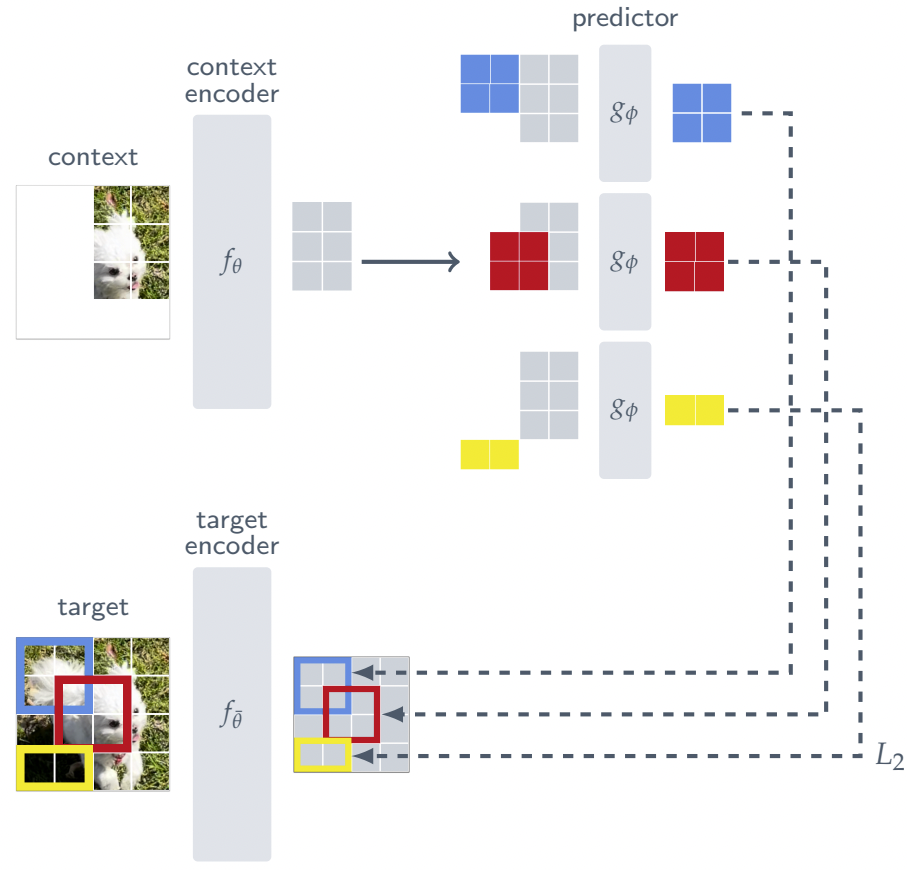
Figure 1. The I-JEPA training architecture, from the paper's figure 3. Matching colors identify the same target region in the two branches. The repeated predictor boxes share their weights; they are not separately trained models.

The order of operations matters. Target regions are selected after the target encoder has processed the complete image. A target feature can therefore incorporate information from elsewhere in that image. The context encoder, by contrast, never receives the hidden target patches as input.

The predictor also needs to know where to predict. Otherwise, the same visible context could be used to ask about several different missing regions. I-JEPA supplies a shared learnable mask token at each requested position, with a positional embedding added to it. These tokens specify locations; they do not reveal the missing pixels. Paper, section 3.

How the networks learn together🔗

The prediction error updates the context encoder and predictor through backpropagation. The target encoder is updated differently: its weights track an exponential moving average of the context encoder's weights.

Think of the target encoder as a slowly changing reference. Each update retains most of its previous weights and adds a small contribution from the newly trained context encoder. The targets improve as training progresses, but do not chase each individual gradient update directly.

This design addresses a risk called representation collapse. If every image produced the same vector, predicting that vector would be easy, but the representation would be useless. I-JEPA uses the asymmetry between the two branches, the predictor, and the moving-average target encoder to train without explicit negative-image pairs. The paper reports that the moving-average encoder is essential in its experiments; averaging alone is not a general mathematical guarantee against collapse.

Why the mask is part of the method🔗

Hiding a few isolated pixels can create a task solvable from nearby color and texture. Hiding almost everything can leave too little evidence to make a useful prediction. I-JEPA instead samples several substantial target regions while keeping context distributed around them.

Its default recipe is:

Sample four target blocks, each covering roughly 15-20% of the image area, with aspect ratios between 0.75 and 1.5. Target blocks may overlap one another.
Sample a square context block covering roughly 85-100% of the image area.
Remove from the context every patch that overlaps any target block.

The 85-100% figure describes the context block before those removals. It is not the fraction of image patches actually passed to the context encoder. The remaining context can have several holes and be much sparser. Likewise, four 20% targets do not necessarily hide 80% of the image, because targets can overlap.

This gives the predictor a different problem from reconstructing scattered pixels: use evidence from visible regions to infer features across several larger missing regions. The paper's masking ablations show that replacing this strategy with random patches or simple quadrants sharply reduces performance in the tested low-label linear-probe setting. Paper, figure 4 and table 6.

Does "no hand-crafted augmentations" mean no cropping?🔗

No. Here the distinction is between constructing multiple transformed views whose representations must agree and constructing a context-to-target prediction task within one image view.

The official I-JEPA pretraining configuration still uses random resized cropping and normalization. Its default recipe disables color distortion, Gaussian blur, and horizontal flipping. The masks themselves are also deliberate design choices. I-JEPA reduces reliance on the multi-view augmentation recipe used by methods such as DINO; it does not eliminate preprocessing or all assumptions about images. Official transforms, ViT-H/14 configuration.

The prediction objective, with the paper's notation

Let $M$ be the number of target blocks, normally four. For block $i$, $B_i$ is the set of patch positions inside that block. The vector $\boldsymbol{s}_{y_j}$ is the target encoder's output for patch $j$; $\hat{\boldsymbol{s}}_{y_j}$ is the predictor's estimate. The collections of vectors for a whole block are written $\boldsymbol{s}_y(i)$ and $\hat{\boldsymbol{s}}_y(i)$.

Section 3 writes the objective as follows, with the equality split across two lines here for readability:

$$ \begin{aligned} &\frac{1}{M}\sum_{i=1}^{M} D\left(\hat{\boldsymbol{s}}_y(i),\boldsymbol{s}_y(i)\right)\\ &\qquad=\frac{1}{M}\sum_{i=1}^{M}\sum_{j\in B_i} \left\lVert\hat{\boldsymbol{s}}_{y_j}-\boldsymbol{s}_{y_j}\right\rVert_2^2. \end{aligned} $$

Read the right-hand side from the inside out: take the difference between the predicted and target vectors, compute its squared Euclidean length, sum over the patches in a block, then average across the $M$ blocks. The paper's displayed expression has a block average and a patch sum; it does not include a separate division by the number of patches in each block.

The context encoder has parameters $\theta$, the predictor has parameters $\phi$, and the target encoder has parameters $\bar{\theta}$. Only $\theta$ and $\phi$ receive gradients from this objective. The moving-average update can be written as:

$$ \bar{\theta}\leftarrow m\bar{\theta}+(1-m)\theta. $$

This last equation spells out the update described in the paper's prose. The momentum $m$ starts at 0.996 and increases toward 1 during pretraining. A larger value retains more of the target encoder's previous weights. Paper, section 3 and appendix A.1.

Paper versus implementation: the released training code normalizes target features and uses smooth_l1_loss with its default mean reduction, rather than the squared-L2 expression printed above. Both train feature prediction, but they are different numerical losses. The equation here follows the paper; reproducing the released checkpoints requires following the implementation.

How it differs from MAE and DINO🔗

All three methods learn from images without needing class labels during pretraining. What changes is the training question.

Method	Training question	Prediction target
MAE	Can visible patches reconstruct the missing patches?	Pixel values, typically normalized within each patch
DINO	Can a student match its teacher across different augmented views?	The teacher's output distribution over learned features
I-JEPA	Can visible context predict features at specified hidden positions?	Patch representations from the moving-average target encoder

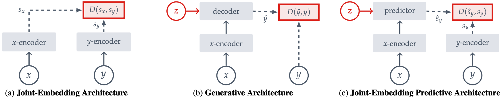
Figure 2. The paper's figure 2 compares architecture families. In the right-hand panel, the predictor estimates a target representation rather than a target image. For I-JEPA, the conditioning information marked $z$ specifies the positions to predict.

The middle and right panels make the central difference visible: a decoder predicts the signal; I-JEPA's predictor predicts its representation. A useful representation need not preserve every detail that a pixel reconstruction requires.

For the reconstruction side of this comparison, see the MAE article. The DINO article explains the teacher-student, multi-view approach.

What happens after pretraining?🔗

Pretraining produces features, not a ready-made classifier for every task. To evaluate those features, the paper uses the target encoder, generally averaging its patch representations into an image-level vector.

A linear probe keeps the encoder frozen and trains a simple classifier on top of its features. This asks whether the representation already makes categories easy to separate. Labels are used to train that classifier, even though they were not used to pretrain the encoder.

Fine-tuning also updates the encoder for the downstream task. It can adapt the representation more extensively, but answers a different question from linear probing. Keeping these protocols separate makes the results much easier to interpret.

Classification: useful features with fewer pretraining epochs🔗

The following results are from the paper's full-label ImageNet-1K linear evaluation, where top-1 accuracy is the percentage of images assigned the correct highest-scoring class:

Method and encoder	Pretraining epochs	Top-1 accuracy
MAE, ViT-H/14	1,600	77.2%
I-JEPA, ViT-H/14	300	79.3%
I-JEPA, ViT-H/16 at 448-pixel resolution	300	81.1%

An epoch is one pass through the training dataset. ViT-H denotes the Huge model; /14 and /16 denote the patch width in pixels. The higher-resolution row processes a different patch grid, so it is not the same computation as the standard ViT-H/14 run.

The matched ViT-H/14 comparison is the clearest result: I-JEPA reaches higher linear-probe accuracy after substantially fewer pretraining epochs. That does not make it the winner over every model in the table: DINO's different ViT-B/8 configuration reaches 80.1%. Paper, table 1.

Low-label learning and spatial information🔗

With only 1% of ImageNet's labels, I-JEPA's ViT-H/14 reaches 73.3% accuracy, compared with 71.5% for MAE's ViT-H/14. This is a separate experiment: the I-JEPA encoder is fine-tuned, not frozen. The 448-pixel I-JEPA variant reaches 77.3%. These results support label-efficient adaptation, not a claim that all downstream tasks need no fine-tuning. Paper, table 2 and appendix A.2.

The paper also tests frozen features on CLEVR, a dataset of synthetic scenes. Its counting and distance tasks check whether the representation retains information beyond object category. I-JEPA scores 86.7 on counting and 72.4 on the distance task; MAE scores 90.5 and 72.4 respectively. I-JEPA therefore retains useful spatial information, but does not surpass MAE on both tasks. These benchmarks should not be read as a demonstration of dense, real-world depth maps. Paper, table 4.

Where the compute savings come from🔗

Meta reports training the approximately 632-million-parameter ViT-H/14 on 16 A100 GPUs in under 72 hours. That is elapsed time for a multi-GPU run, not a single-GPU training budget. At 72 hours, 16 GPUs would account for 1,152 GPU-hours. Meta's June 2023 announcement.

The efficiency comes from several places. The context encoder processes only visible patches. The predictor is narrower than the encoders. The target encoder processes one complete image view rather than a collection of separately augmented views. Most importantly, useful features emerge after fewer pretraining iterations in the reported comparisons.

There is still a cost to generating targets. Section 7 reports that an I-JEPA iteration is about 7% slower than the compared MAE setup; the saving comes from needing fewer iterations. The introduction reports more than a tenfold GPU-hour advantage over its ViT-H/14 MAE reference. That is a comparison of the reported training runs, not a universal tenfold speedup for any model or dataset. Paper, section 1 and section 7.

The distinction is practical: making each training step cheaper and needing fewer steps are different routes to reducing the total bill.

What does it mean to learn a "world model"?🔗

Predicting a hidden region requires learning regularities: which parts tend to occur together, how shapes continue, and what the surrounding image makes plausible. That is the motivation behind connecting I-JEPA to learning through observation.

The evidence here is about spatial relationships in still images. I-JEPA does not learn action-conditioned future states, plan a sequence of actions, or demonstrate general common-sense reasoning. The authors describe the predictor as a restricted kind of world model, not a completed model of how the physical world works.

The image-completion visualizations need one further distinction. I-JEPA itself outputs vectors. To make those vectors visible, the researchers freeze the pretrained model and train a separate generative decoder to produce image samples from the predictor's representations. Structure shared across samples suggests what the representation captures; varying texture shows details it leaves unspecified. Those pictures are a diagnostic tool, not evidence that I-JEPA was trained to generate images. Paper, section 8, official visualizations.

The takeaway🔗

I-JEPA changes both what the model predicts and what it must use to make the prediction. A learned target encoder supplies feature-space targets, while large missing regions and distributed context make the prediction task informative.

The result is a way to learn reusable visual features without pixel reconstruction or an elaborate multi-view augmentation recipe. The paper's strongest evidence is the quality of those features under clearly defined evaluations, together with the training effort needed to obtain them.

I-JEPA addresses learning representations from unlabeled images. For a different stage of the machine-learning workflow, the QLoRA article explains how to adapt an already pretrained language model using less GPU memory. The two articles explore different efficiency questions: learning useful features versus making task-specific fine-tuning more affordable.

Original sources🔗

Assran et al., Self-Supervised Learning from Images with a Joint-Embedding Predictive Architecture, CVPR 2023. The method, equations, and tables discussed here follow arXiv version 3.
Official I-JEPA repository, with training code, configurations, and pretrained checkpoints.
Meta's June 13, 2023 announcement, which places the work in the broader JEPA research program.

Both figures are reproduced from Assran et al.'s paper and retain their original content.