 Michał Chromiak's blog
 Adapting a language model to a new task usually costs much more GPU memory than simply running it. Training needs room for the model, intermediate calculations, and the information used to update its weights. For a model with billions of parameters, those extra costs can put fine-tuning out of reach even when inference fits.
QLoRA combines two ways to save memory: compress the pretrained model and train a small set of additional weights. In their 2023 paper, Tim Dettmers and colleagues use this approach to fine-tune a 65-billion-parameter LLaMA model on a single 48 GB GPU. They also introduce Guanaco, a family of chatbots trained with QLoRA. Paper, introduction.
The method is easiest to understand in two steps: first decide which weights need to change, then reduce the memory used by the weights that stay fixed.
Why fine-tuning needs so much memory🔗
A pretrained model's weights, also called parameters, are the numbers it learned during its original training. Fine-tuning adapts those numbers, or adds trainable ones, using examples of the behavior we want. For instruction tuning, an example might pair a question with a useful answer.
In full fine-tuning, all the model's weights can change. Training also stores gradients, which indicate how to adjust trainable weights, and optimizer state, the running statistics an optimizer uses to choose those adjustments. Activations, the intermediate results produced as inputs pass through the network, require memory too.
The paper estimates that conventional 16-bit fine-tuning of LLaMA 65B requires more than 780 GB of GPU memory. That is a training-memory estimate, not just the size of the model's weights. QLoRA reduces several parts of this memory budget together. Paper, sections 1 and 2.
LoRA: Learn a small update instead of rewriting the model🔗
LoRA, short for Low-Rank Adaptation, keeps the pretrained weights frozen: training does not update them. It adds small trainable components called adapters alongside selected layers. Each layer combines its original computation with an adjustment learned by its adapter.
For example, when adapting a model to answer customer-support questions, the base model continues to supply its learned language capabilities. Training adjusts the adapters using the new examples. The resulting behavior depends on both parts, even though only the adapters change.
An adapter represents an update using two smaller matrices, or grids of numbers, instead of one full-size matrix. Their narrow intermediate dimension is the adapter rank. This restriction greatly reduces the number of trainable parameters and the gradients and optimizer state associated with them. Ordinary LoRA still needs to keep the large base model in memory; QLoRA addresses that remaining cost.
For a fuller explanation of rank, adapter training, and merging updates for inference, see LoRA: Fine-tuning a model by learning a small update.
The algebra: How two small matrices change a layer
The QLoRA paper writes the LoRA computation as follows in equation (3):
Here, \(\mathbf{X}\) is the layer's input and \(\mathbf{Y}\) its output. The frozen matrix \(\mathbf{W}\) has shape \(h \times o\), where \(h\) and \(o\) are the input and output widths. The trainable matrices \(\mathbf{L}_1\) and \(\mathbf{L}_2\) have shapes \(h \times r\) and \(r \times o\). Their product has the same shape as \(\mathbf{W}\), but rank at most \(r\). The scalar \(s\) controls the size of the adapter's contribution.
For an illustrative layer with input and output widths of 4,096 and rank 8, the two adapter matrices contain 65,536 parameters in total. A full 4,096-by-4,096 weight matrix contains 16,777,216. The adapter therefore uses 256 times fewer trainable parameters for this layer. This is a count of parameters, not a prediction of the total GPU-memory saving.
In QLoRA, the base matrix is stored in quantized form and reconstructed approximately for computation. The adapters remain higher precision. The paper's equations (5) and (6) give the full expression, including the reconstruction of quantization scales. Paper, sections 2 and 3.
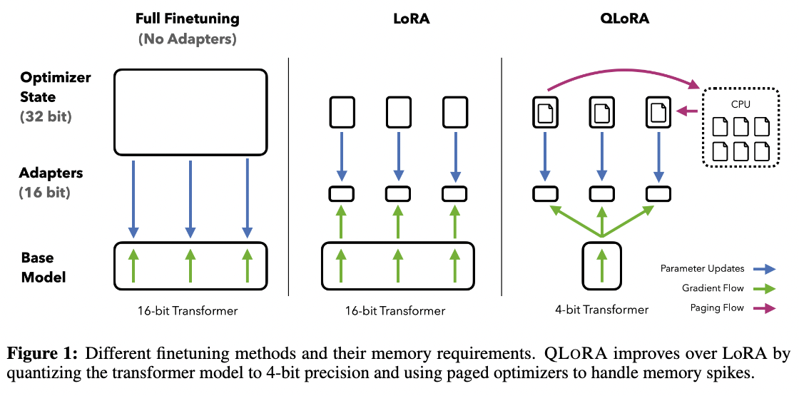
Figure 1. The paper's comparison of the three methods. Blue arrows show parameter updates, green arrows show gradient flow, and pink arrows show movement of optimizer state between GPU and CPU memory. In LoRA and QLoRA, gradients pass through the base model's computation to train the adapters, while the base weights stay fixed. Source: Dettmers et al., figure 1.
What QLoRA adds🔗
QLoRA builds on LoRA with three memory-saving components. Each addresses a different cost: storing the weights, storing the information needed to reconstruct those weights, and handling temporary peaks during training.
1. NormalFloat: Store the base weights in 4 bits🔗
Quantization replaces high-precision numbers with a smaller set of representable values. Four bits provide 16 possible codes. Each stored weight selects one of those codes, which maps to an approximate numerical value.
QLoRA introduces 4-bit NormalFloat (NF4), whose representable values are arranged for a zero-centered normal distribution: a bell-shaped distribution with most values near zero. It places more of its limited precision in that crowded region, where many pretrained weights lie, rather than spacing all values evenly.
The weights are divided into small blocks, each with its own scaling factor. This lets the same set of NF4 values represent blocks with different numerical ranges. The paper finds that NF4 performs better than the other 4-bit formats it tests.
Four-bit storage does not mean four-bit arithmetic throughout training. When the model uses a group of quantized weights, it dequantizes them into a computation format, usually 16-bit BFloat16 (BF16), before matrix multiplication. Dequantization reconstructs an approximation; it does not recover the exact original weights. The adapters learn while operating alongside that approximation. Paper, sections 3 and 4.
2. Double quantization: Compress the scales too🔗
The scaling factors also occupy memory. If every block of 64 weights has a 32-bit scale, that scale adds half a bit per weight. Across billions of weights, this overhead is substantial.
Double quantization quantizes these scaling factors as well. The paper uses 8-bit values for the first set of scales, with higher-precision scales shared across larger groups. This reduces the scale overhead from 0.5 to approximately 0.127 bits per weight, saving about 0.37 bits per parameter, or roughly 3 GB for a 65B model.
The second quantization therefore targets the scales, not a second round of four-bit compression applied directly to the model weights. Paper, section 3.
3. Paged optimizers: Make room for temporary memory peaks🔗
A training run can fit in memory most of the time and still fail on a batch containing long sequences. The extra intermediate calculations create a temporary peak.
QLoRA's paged optimizers use NVIDIA unified memory to move optimizer state between GPU memory and CPU RAM as needed. When GPU memory is under pressure, some of that state can reside in CPU RAM; it returns when the optimizer needs it. This helps accommodate peaks without reserving enough GPU memory for all optimizer state at all times.
Paging works alongside gradient checkpointing, which saves activation memory by recomputing some intermediate results during the backward pass. Neither technique removes the need to budget for sequence length and batch size. Paper, sections 3 and 4.
One training step, from input to update🔗
Putting the pieces together, a QLoRA training step works like this:
- Run the examples through the model. Quantized base weights are dequantized as needed for computation, and the adapters contribute their learned adjustments.
- Measure the prediction error. The model predicts tokens, the chunks of text it processes. A loss measures how well those predictions match the training targets.
- Backpropagate through the computation. Gradients pass through the frozen model's operations to determine how the adapter weights should change.
- Update the adapters. The base weights stay fixed. Paged optimizer state can move between CPU and GPU memory when needed.
This explains how a frozen model can participate in training: its computations influence the adapter gradients, even though training never updates its own weights.
What the experiments establish🔗
The authors compare QLoRA with both full 16-bit fine-tuning and 16-bit LoRA. On the evaluated tasks, QLoRA broadly matches these baselines while using much less memory. The comparison depends on scale: the largest LLaMA experiments, from 7B to 65B, compare against 16-bit LoRA, not full fine-tuning of every weight at every size.
Those LLaMA experiments use MMLU, a multiple-choice benchmark spanning 57 subjects. Table 4 reports mean accuracy of 53.1% for NF4 with double quantization and 53.0% for the 16-bit adapter baseline, averaged across the tested model sizes and tuning datasets. Individual settings vary, but the overall result is close.
Adapter placement matters too. The paper finds that applying LoRA across all linear layers in the transformer blocks is important for matching full fine-tuning in its LLaMA 7B experiment. Adding adapters only to the query and value projections in attention does not achieve the same result. Paper, section 4.
Guanaco and the single-GPU results🔗
QLoRA is the training method; Guanaco is a family of models trained with it. The authors build Guanaco by instruction-tuning LLaMA on OpenAssistant's OASST1 conversation data. They use supervised learning, without a reinforcement-learning stage.
The original release reports two particularly useful hardware reference points:
- Guanaco 33B: fine-tuning on a single 24 GB GPU, with a reported run taking less than 12 hours.
- Guanaco 65B: fine-tuning on a single 48 GB GPU, with a reported run taking about 24 hours.
These are results for the authors' training recipe, not fixed runtimes for arbitrary datasets and sequence lengths. They show how the memory reductions make much larger models accessible on a single GPU. Paper, introduction and section 4; authors' implementation.
What "99.3% of ChatGPT" means🔗
The widely repeated figure comes from Guanaco 65B's score relative to the 2023 ChatGPT baseline in the paper's Vicuna benchmark evaluation. GPT-4 scored responses to 80 prompts; the authors expressed Guanaco's score as a percentage of ChatGPT's and averaged over both response orders to reduce ordering bias. The resulting 99.3% is a relative score under that evaluation, not a measurement of 99.3% of ChatGPT's overall capabilities.
The paper also compares human and model-based judgments and examines failures that aggregate scores miss. Its broader lesson is that the evaluation should match the intended use: strong performance on a multiple-choice knowledge benchmark need not imply equally strong conversational answers. Training-data suitability matters as well as size. Paper, sections 5 and 6.
A closer look: Design choices and memory costs🔗
The following comparisons show where the gains come from. The first tests adapter placement; the second tests number formats; the worked example separates weight storage from the rest of the training budget.
Why does adapter placement matter?
The paper compares several ways to fine-tune LLaMA 7B on Alpaca. Attention layers combine information from different positions in the text. Feed-forward layers, abbreviated FFN, transform the representation at each position. Adapters can be added to either group or both.
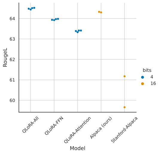
Figure 2. Adapter-placement comparison from Dettmers et al., figure 2. The original figure is linked at full size.
How to read it. Each dot is a run with a different random seed. The vertical axis is ROUGE-L, a measure of overlap between generated and reference answers based on their longest common subsequence. Higher is better on this metric. Blue dots use four-bit base weights; orange dots show the 16-bit full-fine-tuning baselines.
QLoRA-All places adapters across all linear layers in the transformer blocks. It scores above the FFN-only and attention-only variants and is comparable to the authors' tuned full-fine-tuning baseline, labeled "Alpaca (ours)." The lower Stanford-Alpaca results also show why tuning the baseline matters: outperforming a weak training setup would be less convincing.
The useful distinction is where the model can learn an adjustment, not just how few parameters it updates. This experiment supports broad adapter coverage in this setup; ROUGE-L alone does not establish general chatbot quality. Paper, section 4.
What do NF4 and double quantization each contribute?
The paper also isolates the effect of the number format by evaluating quantized LLaMA models. Here, zero-shot means the evaluation supplies no worked examples in the prompt. This comparison tests the quantized models, rather than Guanaco's instruction-tuned conversational behavior.
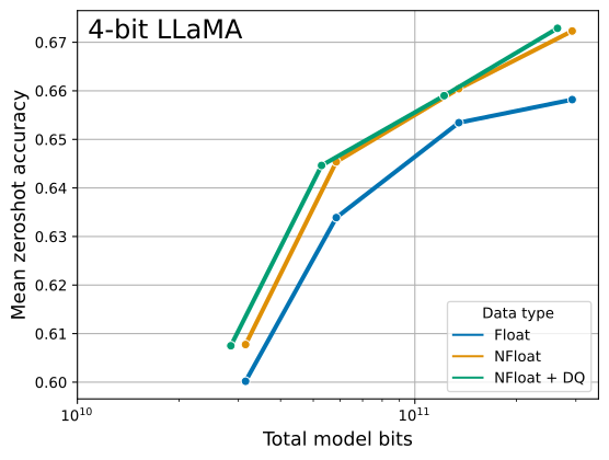
Figure 3. Quantization comparison from Dettmers et al., figure 3. The original figure is linked at full size.
How to read it. The horizontal axis is total model bits on a logarithmic scale; farther left means less storage. The vertical axis is mean accuracy across five benchmarks: WinoGrande, HellaSwag, PIQA, ARC-Easy, and ARC-Challenge. Higher means better performance on that collection of tasks.
The orange NormalFloat curve sits above the blue ordinary-float curve. Both use four-bit weight codes, but choosing the representable values differently changes the error introduced by quantization. The green NormalFloat-plus-DQ curve stays close to the orange curve while shifting left: compressing the scales saves storage with little change in accuracy here.
The two components therefore do different jobs. NF4 improves the representation of the weights; double quantization reduces the overhead of their scales. These results explain the choice of quantization scheme. The fine-tuning comparisons in table 4 address the separate question of how well the models perform after adapter training. Paper, section 4.
A worked memory budget for 65 billion weights
Start with an idealized model containing exactly 65 billion weights. A byte contains eight bits, so storing every weight in 16 bits requires 130 GB. Four bits per weight reduces that to 32.5 GB. These calculations use decimal gigabytes and count only the stored weight values.
| What is stored | Approximate size |
|---|---|
| Weight values at 16 bits each | 130 GB |
| Weight values at 4 bits each | 32.5 GB |
| Four-bit values plus the paper's double-quantized scale overhead | 33.5 GB |
The last row adds approximately 0.127 bits per weight for scales, using the paper's block sizes: 64 weights per first-level block and 256 scales per second-level block. That contributes about 1 GB across 65 billion weights. Without double quantization, the 0.5-bit scale overhead would contribute about 4.1 GB instead. This is where the roughly 3 GB saving comes from. Paper, section 3.
The 33.5 GB estimate is not the total training requirement. A real run also needs adapters, their gradients and optimizer state, activations, temporary computation buffers, and any parameters kept at higher precision. Sequence length and batch size affect several of these costs. Gradient checkpointing reduces saved activations through recomputation; paging lets some optimizer state reside in CPU RAM when GPU memory is tight.
This calculation explains how the frozen weights can fit within the paper's 48 GB training setup while leaving some room for the rest. It is an illustrative storage budget, not a reproduction of the authors' measured peak memory. Their appendix G examines the memory footprint in more detail.
Figures 2 and 3 are reproduced unmodified from the original paper by Dettmers et al., distributed under CC BY 4.0.
The takeaway🔗
QLoRA makes fine-tuning more accessible by separating the large body of pretrained weights from the much smaller set of weights that must change. LoRA reduces the trainable part; NF4 and double quantization compress the frozen part; paged optimizers help handle temporary memory pressure.
The result is a practical route to adapting larger models within a limited GPU-memory budget. The paper's strongest message is the combination: carefully chosen quantization and well-placed adapters can preserve strong task performance without the memory cost of updating the whole model.
Related reading🔗
To contrast efficient language-model adaptation with a spatial foundation model, read Atlas: How one model turns images into controllable 3D worlds. QLoRA changes how an existing model is adapted under a memory constraint; Atlas changes what kinds of observations and structure a model is trained to represent.
For a different approach to training efficiency, see I-JEPA: Learning from images by predicting missing features. I-JEPA learns visual representations from unlabeled images; QLoRA adapts pretrained language models. The articles address different stages of learning, rather than two versions of the same method.
For an architectural example built around dense matrix operations, see MLP-Mixer: How image patches communicate without attention. MLP-Mixer is a vision backbone, whereas QLoRA is a memory-efficient way to adapt a pretrained language model; the connection is computational perspective, not task or method.
Original sources🔗
- Tim Dettmers, Artidoro Pagnoni, Ari Holtzman, and Luke Zettlemoyer. QLoRA: Efficient Finetuning of Quantized LLMs, 2023. This explanation follows the original May 2023 version.
- QLoRA code and Guanaco model information, maintained by the authors.
Comments
comments powered by Disqus